Transcripts
1. Intro: Welcome to the Pandas course. In this course, we
will explore Pandas, one of the most
essential libraries for data analysis in Python. This course will
provide you with the core knowledge needed to
work efficiently with data. We will start by setting up
our working environment using Anaconda algebra and notebook to ensure you had the
right tools for the job. Once that's ready, we will dive into the
fundamentals of Pandas, learning how to
create, manipulate and analyze data frames, the core data
structure in Pandas. After mastering the basics, we will move on to working
with real world datasets, downloaded from open sources. You will learn how
to clean, transform, and organize data, making it
ready for deeper analysis. You will find the download link for the dataset in the
class description. We will also explore multi
indexing and pivot tables, powerful tools for structurizing and summarizing
data effectively. Next, we will cover data
visualization and Pandas, turning raw numbers into
clean and informative charts. We will also learn how to store data frames in a database, retrieve them when needed, and use SQL queries directly in Pandas to interact
with structured data. By the end of this course, you'll be confident
in using Pandas for real world
data analysis from organizing raw
data to extracting meaningful insights.
Let's get started.
2. Getting Started with Pandas: Installation, Anaconda Setup, Jupyter Notebook: Hi, guys. Welcome to
the Pandas course. Nowadays, data is one of the most valuable resources
in the modern world, and being able to manipulate, analyze, and visualize it
effectively is crucial. That's where Pandas, one of the most powerful
Python libraries for data analysis
comes into play. Pandas provides a
fast, flexible, and user friendly way to
work with structured data. Whether you're dealing
with spreadsheets, large datasets or databases, Pandas allows you to clean, transform and analyze
data with ease. It's widely used
in data science, finance, machine learning, and many other fields where data driven decisions
are essential. Mastering this library is essential for
everyone working with data from analysts to researchers and
software developers. One of the main advantages
of using Pandas, its ability to
effectively handle and analyze large volumes
of data thanks to special structures
that make working with data tables and
their analysis easy. Before we start
working with Pandas, we need to do some preparation. First, we will explore the anaconda distribution
and virtual environments. So we can choose what
works best for you. Anaconda is a
distribution of Python. That includes not
only PyTon itself, but also many other
useful libraries and tools for data analysis
and specific computing. One of the main advantages
of Anaconda is that it comes with pre installed
libraries such as Napi, sky Pie, Mud Blood Leap, Jupiter, and of course, Pandas. This significantly simplifies this type of environment for data analysis and allows you to quickly start
working on a project. Conda is a package and
environment manager for Python. That comes with Anaconda. It allows you to install
update and manage versions of Python packages
and other software tools. One of the key benefit of Conda is the ability to create
isolated environments. In these environments, you can install different versions
of Python and its packages, avoiding conflicts between
different projects and ensuring the
stability of your code. Now let's move to practice. First, go to the
installation page and follow the instructions. I will start by
showing how to install it on MacOS and then on Ubuntu. For MacOS, go to the MacOS Installer link
and download the installer. Open the download a file and start the
installation process. Follow the prompts,
allow permissions, agree to the terms, and wait for the
installation to complete. The process will
take a few minutes. Once Anaconda is installed, it will prompt you to update Anaconda Navigator to
the latest version. So let's update it. After updating, you
can immediately start Jupiter Notebook
and being working. At the top, you will see the default virtual environments created by Conda with
all dependencies, so you don't need to install
Pandas. It's already there. You will see the Jupiter
server starting and you can open a document that you already have or
create a new one. As you can see, everything works and Pandas
is ready to use. Now, let's continue with Ubuntu. Go to the Linux Installer link. First, install all dependencies. Then download the installer for Linux. Open the terminal. Run the downloaded file and start the installation by
following the instructions. Agree to the license terms and follow the prompts
from the documentation. When prompted, select yes,
to initialize Anaconda. Next, open the terminal and disable the automatic activation
of the base environment. When installing
anaconda, disabling the automatic activation of the base environment helps avoid unnecessary
clutter in the terminal, gives you more control
over which environment to activate and prevents accidental
use of base environment, especially when managing
multiple projects. This way, you can work in a
cleaner, more flexible setup. Restart the terminal to ensure the base environment
is deactivated. You can list all dependencies using the Conda list command. Finally, launch
Anaconda Navigator. From here, follow
the same steps. Launch Jupiter, open a new file, or already created one, and start working with Pandas. When you open Anaconda Navigator and go to the Environments tab, you will see the base
development environment, that Anaconda created by
default during installation. You can add or delete new development environment or manage the existing
base environment. Here you can see what is
already installed or use the search function to find and install the necessary
packages directly. If you prefer, like I do, to work through the terminal, you can open the development
environment directly from the terminal and install all dependencies using
the P package manager. You can also manage
virtual environments and install Jupiter and Panda
separately without Anaconda. This would be a
completely different way to organizing your workspace. Now, let's get to work.
3. Pandas Series Explained: Creating, Manipulating, and Comparing with NumPy Arrays: So let's get to work. If you decide not to use Anaconda and work with
virtual environment, you can install Pandas using the command Pep Install Pandas. Pandas provides robust
and easy to use data structures that are perfect for data
manipulation and analysis. The main data structures in Pandas are series
and data frame. These structures are designed to handle different types of data and provide
powerful methods for data manipulation
and analysis. A series is a one dimensional
array like object. That can hold data of any type, including integers,
strings, floats, and more. It's similar to a column in a spreadsheets
or a data table. Each element in a series has an associated label
known as an index, which allows for
quick access to data. A data frame is a two dimensional
tabular data structure with labeled axis,
rows and columns. It's similar to
spreadsheets or SQL table. Before we dive into
these structures, it's important to
understand that Pandas is built on top of another fundamental library
in Python called Nam Pi. It's short for numerical Python, and it's library that provides support for arrays and matrices. While a Panda series and numpi array might look
similar at first glance, there are some key differences. A series has an index
that labels each element, making it easy to access data by label rather than just
by integer position. An array on the other hand, only uses integer positions. A series can hold
data of mixed types, while numpi array
is homogeneous, meaning all elements must
be of the same type. Let's import the Pandas
library and check its version. Now let's create a data frame from the data that
we already have. And for this, I create
a list dictionary. List. I will import Napi
and use randint function, which we covered in
the Numpi course. I suggest you familiarize
yourself with it. The random function generates random floating point numbers from the standard
normal distribution. The SID function is
used to initialize the random number generator
with a specific CID value. This is useful for
reproducibility purposes such as in simulations or testing scenarios where
you want to be able to reproduce the same sequence
of random numbers. Now we can see our data frame. It looks like a table
and consists of rows represented by index labels and columns represented
by column labels. Each column is a series. Each element in data frame is accessed using the
row and column labels. In short, a data frame in Pandas can be thought
as a collection of serious objects
where each series represents a column
in a data frame. I removed unnecessary parts. A series and Pandas can be created from
various data types, including lists. We
already have one. So let's create a
series from this list. When creating a
series from a list, Bandas converts the list into one dimensional array like structure with an
associated index. To create a series from a list, you use PD series and pass
the list as an argument. Optionally, you can also provide an index to label the elements. When you don't provide an index, Pandas automatically assigns an integer index
starting from zero. Let's create another series. As a data, I pass X, and as an index, I pass our first
list L. We can also pass arguments
without their names and get the same result. Let's create a series
from a dictionary. If we use such a data structure, we will get a series
where the keys act at the index and the
values represent the data. And here we can clearly
see for the next example, I will create two series that
contains data and indices. Let's consider a situation
where you want to add two Panda series together
using the plus operator. Pandas performs
element wise addition based on the alignment
of their indices. This means that the values
of each index in series one are added to the values of
the same index in series two. We have several
identical indices here, so their corresponding
numbers are added. If an index is present in one series but not in the other, the result for that
index will be none, not a number, indicating
a missing value. One important thing to note is that while we initially
passed integer data, the result contains floats. This is because
Pandas automatically converts integers
to floats during mathematical
operations to handle non values and ensure consistency when combining
different data types. This behavior allows for more flexible and robust
data manipulation seamlessly accommodating missing values
and mixed data types. Let's continue with data frame.
4. Mastering Pandas DataFrames: Access, Modification, Filtering, and Indexing: Let's continue with data frames. I'll start in document and import all
necessary libraries. Let's create our first data
frame with random data. I will generate a data frame with four rows and four columns. To fill this data frame
with random numbers, I will use a function that
generates random values. I will also pass a list as an index and define
column labels. This results in a
typical data frame. To access a column, we use bracket notation
and pass the column name. If we need multiple columns, we pass a list of column names. In fact, we can
perform operations on data frame columns
just like with series, such as addition, subtraction
and multiplication. For example, let's add a new
column to the data frame. I will name it new one, and it will be some of the
columns T and R. As a result, we now have a new column. To delete row, we use
the drop function. For instance, if I delete
the row with Index A, it may seem removed at first. However, if I call
the data frame again, the row A is still there. This happens because Pandas doesn't modify the data frame in place unless we specify parameter in place
equals to true. Setting in place equals to true ensures that the changes
persist in the data frame. Otherwise, the original data
frame remains unchanged. Similarly to drop a column, we use draw function, but need to set the axis
parameter equals to one. Since the default axis equals to zero refers to row deletion. I add in place equals to two so that the changes
take effect immediately. And here we deleted the row, and if I specify axis equals to zero,
nothing will change. This is the default value. The shape attribute
returns a tuple that indicates the number of rows and columns
in the data frame. It's useful when you
need to quickly check the size of data frame or
validate data dimensions. Rows can be selected by passing the row label to
the log function. Remember, for
selecting a column, we don't need log function. We can simply use
bracket notation. If we want to select rows using integer based
indexing, we use Iloc. This allows us to
retrieve rows based on their numerical position
regardless of their named index. For example, using IoC zero, we will return the first row. For convenience, I will
display our data frame again. To extract a specific
subset of rows and columns, we use log function and pass both row and column labels
using a coma notation. If we want a subset of specific rows and
specific columns, we pass two lists, one for rows and
one for columns. And here we can see the
subset of RT column, and as zeros, there
are many situations where we need a subset of data that meets
certain conditions. And for that, Pandas provides
filtering capabilities. Pandas allows for
conditional selection to filter data based on
specific conditions. For example, if
we want to select all data values
greater than zero, the output will be a
filtered data frame where non matching records are replaced with none,
not a number. Now let's try column
based filtering. I will extract data based on condition where E column has
values greater than zero. Initially, the output
will show Boolean values, true where the condition is
met and false otherwise. To retrieve actual data, that meets the condition, we must apply the condition
directly to the data frame. This will return only rows where the E column has value
greater than zero. If we modify the
condition, for example, selecting values
greater than one, the output will reflect this
new condition accordingly. The reset index
method allows us to reset the index back to the
default numerical index. When we reset the index, the old index is added as a column and new sequential
index is created. The set index method
allows us to set an existing column as the
index of the data frame. Here I took the T column
and use it as an index. Using Python's built
in split function, we can effectively
generate a list. We can generate
list in such a way. It takes much less time item of several values to
be equals to three. And then add this list as a
new column in our data frame. The split function
in Pandas is useful for separating strings
into multiple parts based on a delmeterEtracting
specific data or creating new columns
from text data. If no separator is specified, the split function splits the
string by any white space, spaces, tabs, or new
lines, like in our case.
5. Working with MultiIndex in Pandas: Hierarchical Indexing Explained: As always, let's import
all necessary libraries. The multi index or
hierarchical index is an advanced version of the
standard index in Pandas. You can think of it as
an array of tuples where each dapple represents a
unique index combination. This approach allows for more complex
indexing structures. Let's start by creating
a simple data frame. We will then generate a hierarchical index using
the from frame function. This example will help
us understand how to create a hierarchical
index from a data frame. Let's start by creating
a simple data frame. First, we create data frame with a list of data and column names. This data frame will later be used to construct our
hierarchical index. I pass a list of data
and column names, and our data frame is ready. Now we have a
typical data frame. It includes an index, column names and data. This data frame will be used
to create an index object. We use the From frame function and pass our data
frame as an argument. Now we have an index object, which represents a
list of unique tuples. So let's create a new data frame using this finished multi index. First, I fill out the data
frame with random numbers. Next, we define a structure with four rows and two columns. We pass the multi index
at the index parameter. Finally, we define column
names for the new data frame. And now we can see
the new data frame. We used from frame to create a multi index from a data frame, enabling hierarchical
indexing for better data organization
and efficient selection. And now we can create new data frame using
this multi index. But when creating
a new data frame, the number of rows in
the data must match the number of index levels
to avoid size mismatches. Now I will show
you how to create and work with an index in
a slightly different way. First, I use Python's
split function to create list faster. Then I use the Z function to connect each pair
of items together. Finally, I convert them
into a list Taples. The Z function in Python pairs elements from
multiple iterables, creating tuples of
corresponding elements. It's useful for iterating over multiple sequences
simultaneously. Now I can create a multi
index from an array of taples using the
from Taples function. So we have our multi index and we can integrate it
into a new data frame. First, I fill the data frame with random data
as we did above. Next, I define the structure with six rows and two columns. Then I pass our multi
index, the index attribute, and finally, I define the
column names. Here it is. We can see our new data frame. Okay, let's consider accessing
data with multi index. Using the names attribute, we can set names for the
levels of the multi index. And here I set the names for
our multi index columns, units and workers.
So let's practice. For clarity, we can see two marked columns,
units and workers. To get the salary of worker
three from Unit two, I use the log function. First, I indicate Unit two, then I specify Worker three, and finally, select
salary column. The double lock is used because data frame
has a multi index. The first log with Unit two selects all rows under Unit two, returning a smaller data frame. The second log, worker three, then selects Worker three from
this subset, and finally, salary retrieves all
specific column value, and now we have
the result, 0.48. Let's try another example. Getting working hours for worker one and Worker
two from Unit two. You can practice on your own. Post the video and try
doing it yourself. I use log function for Unit two, then I pass Worker one
and Worker two as a list. And finally, I indicate
the hours column. I pass worker one
and Worker two as a list within a list to
select multiple rows at once. This allows us to retrieve
the hours columns for both workers simultaneously from the subset of data
under Unit two. And now we have the working
hours for these two workers. Ignore the negative values since we filled the data frame
with random numbers. Real world data would
contain valid values. Now let's practice to select
multiple rows and columns. What do we need an intersection of several rows and
several columns? Let's get salary and hours for Worker two and Worker
three from Unit two. First, use Log function
to select Unit two. Then pass Worker two and
Worker three as a list. Finally, select salary
and hours also as a list. So pause the video and
try to do it yourself. As you can see, we
used the same method, the function and
bracket notation. Then define Unit two
at the first level, passing worker two and
Worker three as a list, and finally passing
two list of columns, salary and hours using
bracket notation. I can avoid passing columns, salary and hours as a list because we only have two columns
in our data frame. In this case, all columns will
be selected automatically. These two versions will
give the same result. However, if we had
more than two columns, we would need to explicitly
list the column names. So this was a short example of how to work with hierarchical
indexing in Pandas. The main goal of this lesson
is to understand what hierarchical indexing
means and how it integrates with Pandas
indexing functionality. Multi indexes are
useful in Pandas, but are not always
the first choice. They are commonly used in
hierarchical datasets, time series analysis, and when working with grouped
or pivoted data. However, in many
practical cases, a flat index with
multiple columns is preferred for simplicity
and better readability. So don't be afraid.
In most cases, we won't need to use it, but it's essential to understand its structure and how it works.
6. Pandas DataFrame Analysis: Grouping, Aggregation, and Math Functions: Now I want to introduce you
to a new method in Pandas. And for this, I will
create a data frame. As always, at first, I import the Pandas library. Then I create dictionary. And then from this dictionary, I will create the data frame. The head function on Pandas returns the first few
rows of data frame, typically used to quickly expect the top
position of the data. By default, it shows
the first five rows. Filtering rows and columns in the Pandas library can be
done using filter method. By using Shift plus top command, you can expand and view the conditions under
which we can filter. This method allows you to
select rows and columns based on certain conditions
specified by the user. As a result, we get
data frame with rows or columns that meets
the specified conditions. It's important to
note that filtering only applies to the
index or labels. The data and data frame
itself is not filtered. In this case, when
filtering with the items parameter and
passing the names our columns, name or age, we get only
the requested data. If the items parameter
is specified, it allows you to indicate
a list of columns to keep. If not specified, all
columns will remain. Now I will demonstrate the
example using the parameter. This parameter allows
you to specify a substring that must be
part of the column name. Only those columns whose names contain the string will be kept. If I check it, we
can clearly see it. There is also the
axis parameter. This parameter indicates whether to apply filtering to rows, axis sequLs to zero or columns, axis sequLs to one. To make this clearer, I will add some unique values instead
of the standard indices, which can be read and filtered based on the
certain criteria. After reloading the rows
using Shift plus Center, let's see how this works. I want to get rose that
contains the substring BL, so I will specify
parameter equals to BL and X is equals to zero. This will return
only the row with the index blue and all the
necessary information. Sometimes it's useful to sort the data frame by the value
of one or more columns. The sort values function
is very useful for this. You specify the
column name or list of columns by which the
sorting will be done. For example, here, I
sorted by the column age. For ascending order, the ascending parameter
is set to true. If you want to descending
order, set it to false. Additionally, if you want to change the original
data frame directly, you need to set the in
place parameter equals to true as we did previously. By default, it set to false. If you change the data frame
and then call it again, you will see that nothing has changed unless we set in
place equals to true. For the next example, I will
import the Seaborn library. I'm using this
library because it allows me to load
the Titanic dataset. Yes, Seaborn has default
dataset that I can load. Now I will load the
Titanic dataset and display it so we can
see the available data. Seborn is the PyTon library used for statistical
data visualization. It simplifies creating informative
and attractive charts, making it easier to explore
and understand data patterns. You can find a tutorial for
this library in my profile. Welcome. Let's get acquainted
with group by method. The group by method is
used to group rows in a dataset based on the values
of the one or more columns. Let me give you an example so you can understand
how this works. In this example, I will group all people of the
ship by their class. When I display the result, we get a group by object. I grouped the passengers
by cabin class, and now I want to calculate the average fare for each class. I use the mean
function to do this. Take a look at the result. We can see a large gap. First class is very expensive. Second class is more affordable, and the third class
is the cheapest. Additionally, we can look
at the maximum fare for each class or the minimum fare. However, the minimum
fare shows zero. Let's check if there
are such data. So passengers may have
traveled for free, or we might have missing
data on this data frame. But that doesn't affect, for our example, is
just for demonstration. Let's continue with aggregation. Aggregation is the process
of calculating one or several statistical metrics for each group formed
during data grouping. Data grouping is done
using one or more keys, columns, and then aggregation is performed separately
for each of these groups. Now that we are familiar
with group by method, we can apply aggregation
function like sum or mean to the grouped data. For example, I grouped
the passengers again by cabin class and then calculated the average age
of passengers in each class. Here we can see the correlation. The lower the class, the
younger the average age, which logically makes sense. In those times, older people
were often wealthier, so they traveled
in higher classes. Now I will give you an
example using the egg method. This method, short
for aggregation, is used to calculate
aggregate statistics for groups of rows formed
using the group by method. I grouped the passengers
by cabin class again. Now I want to calculate
the average age and average fare for
passengers in each class. This notation is equal
to what we saw above, but written in a
more compact form. We use the Ag
method to calculate both the average age and
average fare in one line. If you want, the egg method can also make multiple
aggregation functions. For example, you can calculate both the mean and
max for each group. The result will include
all the requested metrics, providing a broader
view of the data. If you're using
multiple functions, don't forget to enclose them in square brackets
because it's a list.
7. Working with Real Datasets: Data Downloading, Analysis, and SQL Integration in Pandas: Now that we've covered Bonds, it's time to solidify our knowledge by working
with real datasets. I will show you where you can find real data for
your projects. If you want to practice
more independently, I highly recommend doing so. Notutorial or video
can teach you more than hands on experience
with real world data. So let's consider bad
sources for real datasets. And the first one Cagle. This is a platform where you can freely download datasets, explore notebooks, and learn
from other data enthusiasts. It's one of the
best resources for data analytics and machine
learning projects. The second one data world. It's another great resource
where you can find datasets on various topics and download
them in multiple formats. Next, we can use
data playground. This site allows you
to browse datasets by topic and format
before downloading, making it easier to
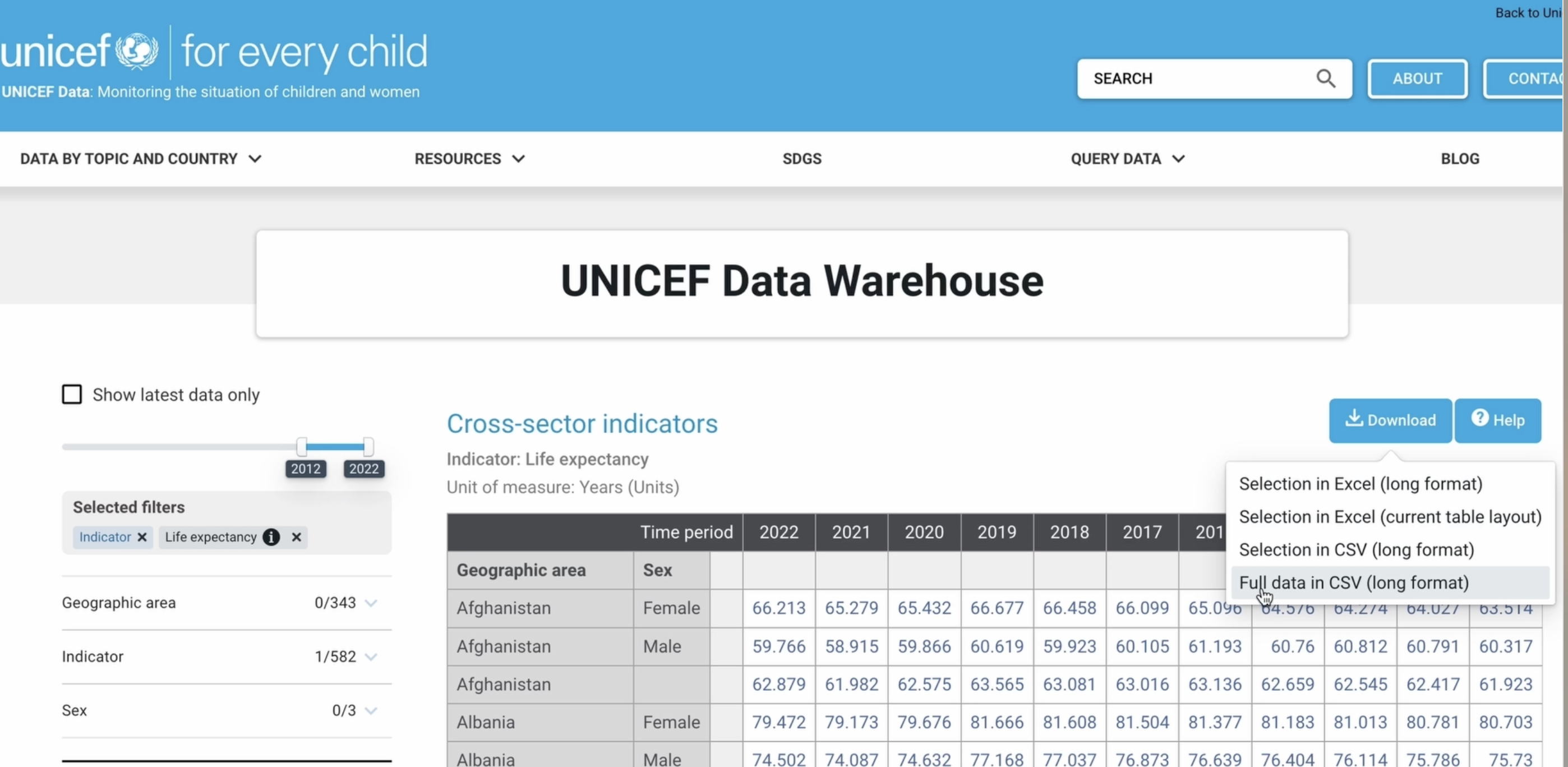
find relevant data. You want to work with
real world statistics, UNICEF provides datasets related to global development,
health and education. These resources is very useful, especially if you want
to create a pet project that reflects the real state of things of a selected topic. For those who don't know, a
pet project is a project, you do at home to showcase in an interview or simply to practice and to understand
how things work. Many governments provide
open data portals where you can download
datasets on real estate, health, finance, and much more. I went to a government
open data website. And I decided to
download a dataset containing information of
real estate sales 2001-2020. I downloaded the
dataset in CSV format, which contains data on real estate transactions
over the years. This is the dataset I will
be using for our project. First things first, I'm port Pandas and use the read CSV method
to load the dataset. Since I'm in the same
directory as the dataset file, I don't need to specify a
full path, the file name. When you try to load large
dataset into a data frame, Pandas attempt to automatically determine data types
for each column. However, for large datasets, this process can consume a lot of memory and usually
takes a long time. To avoid this, you
have two options, manually specified
data types for each column using the
D type parameter or set the parameter low
memory equals to false to allow Pandas to use more
memory for better performance. Since our dataset contains
almost 1 million rows, it's not surprising
that we received a warning message
when loading it. When you load a large dataset and you want to see
what it looks like, you don't have to display
the entire data frame. The head method allows you to review only a portion of it. Similarly, you can view
a specific number of rows from the end
using the tail method. The info method helps you get an overview of
your data frame, including many information like total numbers of
rows and columns, count of non null
values in each column, memory usage, and other. The describe method provides a statistical description of numerical data in
the data frame. From this, you can easily get a general idea of the distribution and statistics of your numerical dataset. It includes mean
standard deviation, minimum, maximum
quartiles, and more. There is also a
powerful Python library called SQL alchemy, which allows you to work with
SQL databases in Pandas. It's particularly useful if you want to store
or retrieve and process large datasets
effectively using SGWL queries. SQL alchemy is a popular library for interacting with relational
databases in Python. SQLite it's another option, which is embedded high performance relational
database management system that it's easy to use and doesn't require
separate server. It allows data storage
and management in a local file store without the need for
separate data server. Well, don't be intimidated
by this code. It's standard. You can simply copy it
from the documentation. All you need to do right now
is understand what it does. Here we import and create an engine to connect
to the database. Suppose you need to
transfer data from a Pandas dataframe
to a database, where you can work
with it further or store it for future analysis. I will demonstrate
how to do this. We've created an engine
connected to the test database. Let me remind you that your
data frame looks like this. Here it is using
the two CSV method. We then write our
data to a table, which I named New table. The second parameter, of
course, is our engine. As we can see, we just saved almost 1 million rows to the new table in
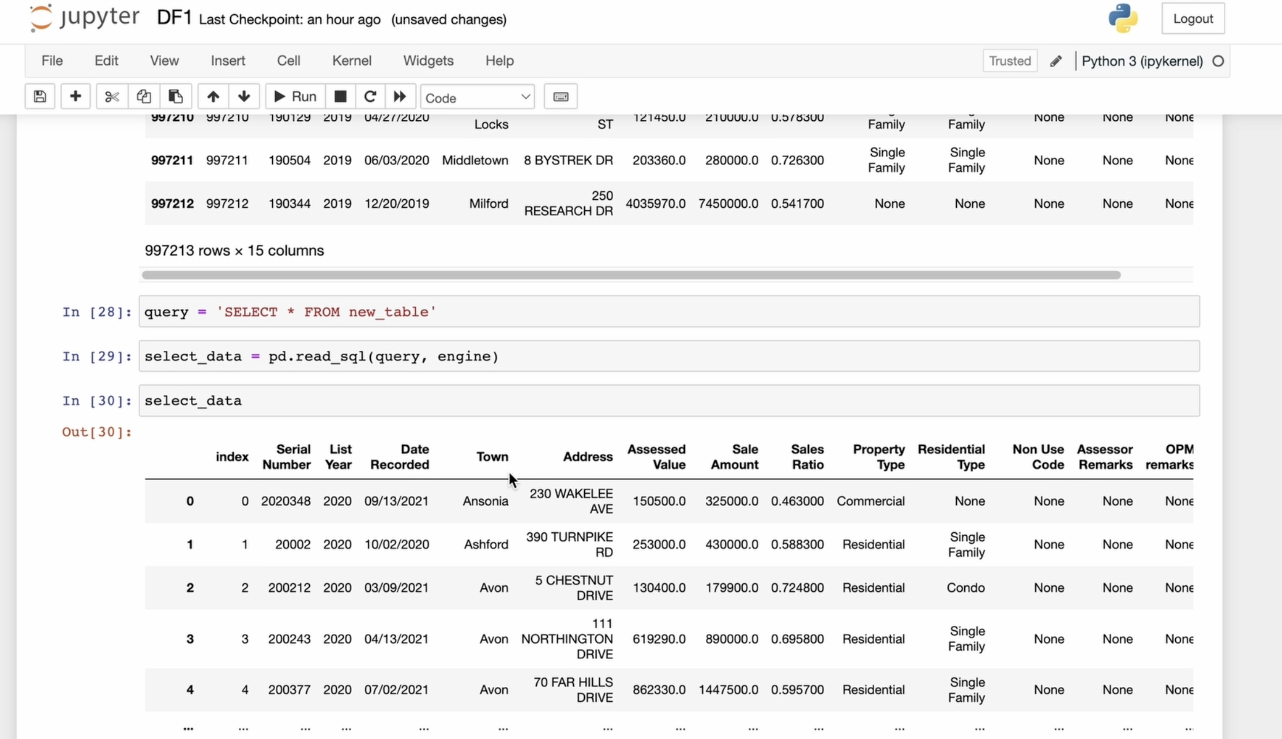
the test database. Let's try to read everything
we saved into this table. In other words, we
want to extract and get our data frame that we
just saved in the database. For this, I use
read SQL and plus our table from
which we intend to read everything at
the first parameter. The second parameter is the engine through which we are connected to
the desk database. I save our extracted data
frame in the read DF variable, and we can see what we
saved in the database. And then we were
able to retrieve it. Here it is. But let's
not dwell on this. We can read not only
the entire data frame from the database
where we saved it, but also take a specific parts with which we plan to work. Now I will show you
how we can form SQL queries before passing
them as a parameter. Knowing how to work
with SQL queries is very useful for everyone, whether you are data analyst
or software developer. The skill will come in handy. The first and simplest query, I will read all the
records from table, and the asterisk symbol means
I'm selecting all records. Then I pass this query and the first parameter
to the same function we used for reading. Of course, the second
parameter is the engine, which is our connection
to the database. It will take a little time. Essentially, we get the same
thing for entire data frame. Now, if I replace the
asterix with town, I will not get the
entire data frame. I will only get
that selected rows. I will get only
what we selected. In my case, it will be cities. To better understand
how it works, let's try something else. I want to retrieve all
information from our data frame, but only for a specific town. Let's say Ashford. And look, we got
information about real estate sales related
only to the town of Ashford. It's convenient, and you
don't need to drag along unnecessary information
in your data frame if you only need to work
with a particular town.
8. Pivot Tables in Pandas: Data Cleaning and Real-World Data Analysis: When we get data that we
need to process or analyze. In most cases, we can't
start working with it immediately because
it's raw data. The outcome we obtain
will be directly influenced by whether
each column was filled with the
appropriate data type and if there are any
empty or zero values. When we receive data,
an initial analysis is extremely necessary. The INL command helps identify missing or zero values within
the data frame object. It returns a new data frame of the same size as the
input data frame where each element is true if the corresponding
element is missing or zero and falls otherwise. This method is very useful for cleaning and analyzing
data because it allows us to identify places where the original
data has missing values. Let me remind you what your data frame looks
like after using INL. To handle these missing values, we can use various methods. For example, fillna allows us to replace empty values
with a specific value. In my case, I used zero. Special attention should
be given to column names. Using columns, I can retrieve all column names as a list
and assess their validity. In many cases, renaming columns is desirable for better
readability and usability. This includes removing
unnecessary quotes, eliminating extra spaces, converting all columns
named to lower case, and replacing spaces
with underscores, if a column name consists
of two or more words. Let me start with a
simple Python example. Suppose we have a
variable A containing the string Nick and we apply
the lower method to it. This transforms all letters to lowercase, resulting in Nick. However, simply
applying this method to data frame columns is not possible as column names are not directly
treated as strings. If we check the type and
first case and in the second, we can see the difference. To process them correctly, I use the STR accessor which enables string operations
for each column name. So what we are doing here, the first one adds access
column names using SDR then convert them to lower
case using lower method. And finally, replace spaces with underscores
using replace method. This approach allows us
to efficiently clean column names without using
loops or manual naming. We can reduce the number
of lines and execute all sequential commands in a single line using
dots notation. It's called method chaining. After performing
these modifications, I have to reassign the processed column names
back to the data frame. This process is
called data cleaning. Here we replace empty values, standardize column
names for convenience, and prevent potential errors
in future data processing. Since I didn't specify
the parameter and place equals to true when filling
in the missing values, you can see that they
are still there, but you can easily replace
them with zero yourself. Just run fill N again and
make sure to save the result. Another important
method is dropna, which is used to remove
rows or columns from a data frame that contains
missing or zero values. By default, if no additional
parameters are specified, drop NREMs rows that
contain missing values. However, this may
result in all rows being deleted if any
column has missing values. To specify whether we want
to drop rows or columns, we use the axis parameter. Axis equals to zero, default removes rows, and axis equals to
one removes columns. For example, setting
axis equals to one will delete columns
instead of rows, producing a completely
different result. How can we identify
unique values? And for this, we
use unique method. It's useful for identifying distinct values in a
specific data frame column. This helps in analyzing
categorical data, such as counting the number of different categories or unique
identifiers in a dataset. For example, to
determine the number of unique cities in
the town column, I will use DF then town in bracket notation
and the method unique. And we got the result. Unlike unique and unique
method counts the number of unique values in each
column or row of a data frame helping to
analyze data distribution. Here we have 18 unique towns. Another useful method
is value accounts, which counts the occurrences of each unique value in
a data frame column. It returns a series where unique values are
listed as indexes, and their counts appear
as corresponding values. This method is
particularly helpful for understanding the distribution
of categorical data, identifying the most
common categories, and analyzing the frequency
of unique values. For instance, using
value accounts on the town column allows us to see how many times each unique city appears
in our data frame. And now let me introduce you to the concept
of pivot table. A pivot table is used to create a summary table from data
contained in a data frame. It helps group and
aggregate data according to certain criteria and arranges it in a format that is
convenient for analysis. As a result, it gives us a handy table for further
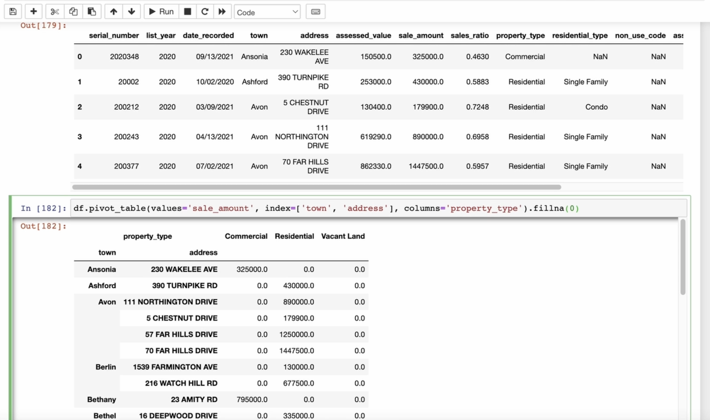
analysis and visualization. I will create a pivot
table from our data. I will use the sum of sales, add the value and for the index, I want to see the
city and address. For the columns, I will
use the property type. Look at the table we have now. We can now work only
with the data we need. Let's refine it further and
fill in the empty values. And now that we have
refined our data, we can move on to other tools. In principle, 90% of your work will involve
what we just did. Pandas is widely used for data manipulation, analysis,
and visualization. It's great for filtering
grouping and reshaping data, as well as performing calculations
like sum and averages. It's also essential for working with time series data and for summarizing information
using functions like describe or Pivot table. Let's also explore data
visualization and Pandas.
9. Pandas Data Visualization: Charts, Graphs, and Insights: Data visualization
is the process of creating graphical
representations of data to understand the structure and identify patterns, trends,
and relationships. We can use various
charts, diagrams, and other visual elements to convey information and
facilitate data analysis. Which format of data is
easiest for you to perceive. If I show you information in a tbar format versus
a visual one. The visual format is
undoubtedly more user friendly and easier
to understand. Visual analysis can also
help identify anomalies, outliers, and unexpected
patterns in the data. Pandas, which we've
discussed earlier, has built in tools for data visualization based
on the Matlot Lip library. Mat Blot Lip is a
Python library for data visualization that
provides a wide range of features to create
various types of charts and diagrams for data
analysis and display. I want to reiterate
that Pandas and Matlot Leap are two
different libraries. The built in
visualization tools and Pandas are based
on Matplot leap, but they provide
a higher level of abstractions and
simplify the process of creating simple charts. The choice of library depends
on your specific needs. If you need to quickly
visualize data in Pandas data frame
using simple syntax, the built in
visualization tools in Pandas may be more convenient. If you require more control over the charts or need to create
more complex visualizations, Matlock Leap might
be better option. Often both libraries are used depending on
the specific tasks. Let's start with the simplest
built in tools in Python. As always, let's
import everything we need and create a data
frame with random data. The main method for
visualization is plot, which can be called on data
frame or series object. I created a data
frame and filled it with random numbers
using the Numbi library. As a first example, let's plot a line chart
for all columns. In the latest versions
of Jubter node books, you generally don't need
to use such commands like PLT show or Mtlot leap in line
for simple visualizations. Mutlot leap in line, and this magic command
is automatically applied in newer version
of Jupiter node books. So charts will be displayed in line by default without
needing this command. Many cases, calling PLT show
is not necessary either. In Jupiter notebooks,
plots are displayed automatically after a
plot command is executed. However, if you want to control, when the plot appears like in scripts or
other environments, you might still use PLT show. So for most basic plotting
tasks in Jupiter, you can simply
create plots without needing these commands
if you're working in a different environment or a Python script outside
the notebook and want charts to be displayed automatically without
needing call PLT show, you can use this configuration. Next, let's create a
histogram for column A. I will call plot and build a histogram on the series
of our data frame. I can change the Bins parameter, which controls the number of
columns in our histogram. By adjusting the number of bins, I can get either a more detailed or more general
view of the data. Next, let's build a scatterplot. Scatter plots are often used to identify correlations
or compare groups. They help us see how
two variables interact. In our case, since
I have random data, it won't reveal much. But with real data, which we covered in
the previous lesson, scatter plots can provide
valuable insights. Now I will show you
how to create by chart based on data
from a series object. First, I create the series
and then build the chart. We use the Pipe method, which generates a pie chart based on the values
of our series. You can also display
the percentages of each part of the Pi. In this case, I display the percentages with
one decimal place. Pie charts are typically
used to visualize proportions or the
percentage relationships between different categories. Next, let's look
at the box plot. Boxplot are used to visualize
the distribution of data showing the
median quartiles, minimum and maximum values. They can also help detect
potential outliers. You can arrange the
boxes either vertically or horizontally by setting
the vert parameter. Additionally, we can
customize the colors of the boxes caps, let it be gray lines representing the
medians and whiskers. The area plot shows
the data in a form of stacked areas for each
column in data frame. If you set the
stacked false option, it prevents the areas
from overlapping and instead shows the
aggregated values for each column separately. This is useful for comparing how much each column
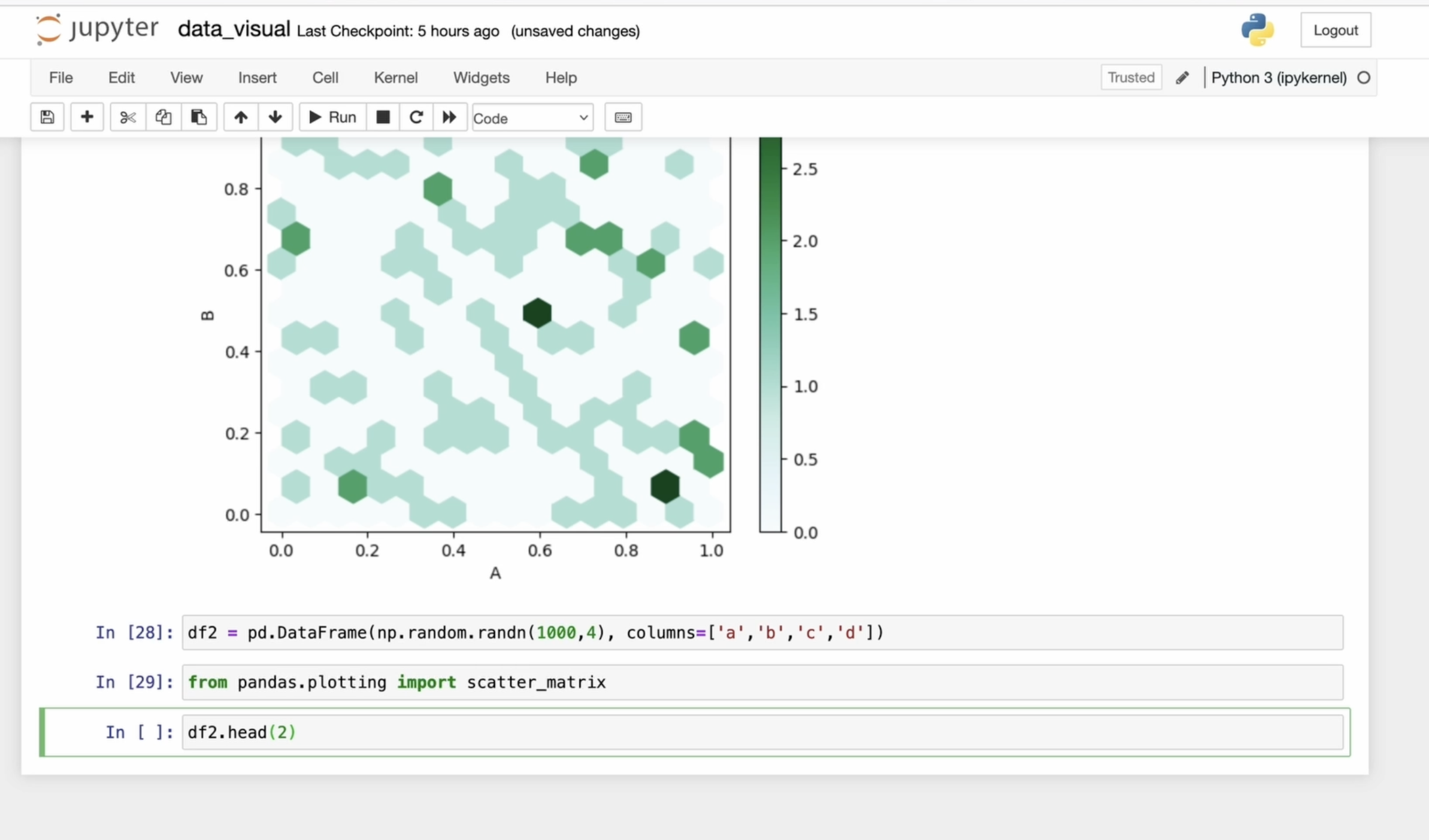
contributes to the total. Next, I will show you how to
create Hg Bin scatter plot. We use the Hg Bin method
to create this plot. The grid size parameter specifies the number of
hexagons used in the plot. A higher grid size leads
to a more detailed plot, but can make it
harder to interpret. Hexbin plots are
great for visualizing the density of data points
in a two dimensional space, especially when you have
a large number of points. Let's also explore creating
a scatter plot matrix. A scatter plot matrix visualizes relationships between multiple
columns of a data frame. For this, I created, again, data frame with
the umpire library. Methods, like we used before
like scatter area, box, and other are available through plot and
Pandas because they are built in Mud plot
leap integration for basic visualizations. However, scatter plot matrix
requires a separate input, since it generates multiple
scatter plot at once, making it more complex than
standard plot methods. So I call scatter matrix, pass our data frame. You can adjust transparency with the Alpha parameter 0-1.
Set the figure size. It sets the figure
size to six by 6 ", determining the overall
dimensions of the plot for better readability
and layout control, and use kernel
density estimates on the diagonal for a
smoother visualization. Each plot on the diagonal shows the distribution
of each column. Scatter plot matrices
are useful for simultaneously
comparing all pairs of variables in a data frame, helping to identify correlations and complex dependencies. While generating
scatter plots for every combination of variables can be computationally
intensive, the scatter plot
matrix simplifies this process and allows easy
analysis of large datasets. Well, we've covered most of what Pandas offers for
data visualization, but there are still
more tools and libraries available to
assist with this task. In the Pandas ecosystem, several libraries can
help with visualization, and you can choose according
to your preference. Congrats on completing
the course. You now have a solid foundation in Pandas for data analysis. If you want to go further, check out my tutorials on
Mud Blot leap, seaborne, and StreamltT advance your visualization
and building skills, keep learning and see
you in the next course.
 Olha Al, Software engineer