Transcripts
1. Intro: Hi, guys. Welcome to
Discourse on Mastering Nampi, one of the most essential
libraries in Python. If you are interested in data science or
machine learning, then Nampi is your
starting point. It's the foundation for so many powerful Python
libraries like Bandas, modo Leap, and psyched learn that are widely used
in the industry today. NumPi is the backbone of data manipulation and
numerical computing. It's incredibly fast and
efficient for handling arrays, performing mathematical
operations, and manipulating data at scale. Whether you are
calculating statistics, building machine learning
models or creating simulations, Numpi will be your go to too. So who needs Numpi If you're aiming for roles
like data scientist, machine learning engineer,
or data analyst, these libraries must
have your toolkit. Understanding Nampi
will give you the skills to handle datasets, process large amounts of data, and build a strong foundation
for more advanced tools. This course is designed
for beginners, so don't worry if you're
just starting out. All you will need is a basic understanding
of Python and ensure that Jupiter notebook or ID like Pycharm or
VSCode is installed. I'll guide you step by
step through everything. In this course, you will learn how to create and
manipulate rays, perform basic mathematical
and statistical operations, Master the core techniques for working with
data efficiently. By the end of this course, you'll have a solid
understanding of Napi and the confidence to use it
in real world projects. Even more importantly,
these skills will serve as a gateway to mastering data analysis and other advanced
Python libraries. Throughout this course, I highly recommend that you take an
active approach to learning. As we go through each lesson, feel free to pose the video and practice the
code yourself in your Jupiter notebook
or Pi harm or viscod. Try rewriting the code you see on the screen and
experimenting with it. Test how each function works. Change some values and see
how the results differ. This hands on practice
is key to really understanding how Numpy works and becoming
comfortable with it. Remember, the best way to
learn programming is by doing. So don't just watch
all along with me. This will not only help
you build confidence, but also ensure you truly
grasp the concept we cover. So let's dive and start
building those skills.
2. Python Installation: And first, let's check if Python is already
installed on your system. If you have Windows, you can do this by
pressing Wind plus R and typing CMD
and hitting Enter. In the command prompt window, type the following
command and press Enter. And here we are, we
can see our Python. On MacOS and Linux, we also open terminal Window and type the following command
and then press Enter. Don't pay attention all
these Python versions. We'll cover it later.
As we can see, I don't have the
command Python version, but I have Command
Python three version. The commands Python version
and Python three version are used to check the version of the Python interpreter
installed on your system. Python version, the command traditionally used to check
the version of Python two, while Python three version is specifically used to check the version of the Python
three interpreter. Typically, Python two was
used on older systems. If you prefer, you can adjust your system configuration to make Python point
to Python three. But I prefer continuing with the command Python three because
it's commonly practiced. If you don't have any Python
on your operating system, we will go to the python.org site and
follow the instructions. Here you choose your
operating system and choose version
of Python you need. I work on MacOS and Linux, but installing Python on Windows is not much
more difficult. You download the
version of Python, then open download it file, and follow the
installation prompts. Here we can download
Python for Linux. If we go to Python, Python packaging user guide, and here I choose tutorials and then choose
installing packages. We can see a lot of information how to check the version of Python and also how to install Python on different
operating systems. And here you can notice that we can install Python
in different ways. For example, here we can see
the commands we can use for installing Python on a
Bunto or if we use MacOS, we can use Homebrew. Homebrew it's a package manager. You can read more on its site. With this package manager, we can install Python
using this command. But what the difference?
Well, shortly, the folder, Homebrew and official installer use the different folders
for installation. Also updating. Homebrew
easily update Python to the latest version with a single command
Brew upgrade Python. Homebrew also
manages dependencies and automatically
cleans up old versions. While official
installer to update, you need to manually
download the new version from the website and go through the installation
process again. The installation via
the official installer is more self contained, which may be useful
in certain scenarios, but can make managing
dependencies and additional tools
more cumbersome. And it often adds application icons in the
applications folder. If I want to see all
Python versions, I installed with the command
Brew install Python, I can use the Command
Brew List Python, and I immediately see all folders and all
Python versions I have. Also, I want to notice
that uni installation with Home Brew is
straightforward with a single command Brew
Uni Install Python, which completely removes the installed version
from your system. While official installer
uninstalling is more complex and require manual removing files from various directories. As for me, Homebrew is more convenient for
developers and those who frequently work with Python and other tools via the terminal. Official installer might be
suitable for users who prefer minimal system interference and need to install Python
once for specific needs, and don't plan on frequently updating or managing
multiple versions. The same thing if we use
Linux, Ubuntu, whatever, we can use Sudo Ogat install Python or we can installing
Python from source. In the first case, this is the simplest method
to install Python, but you can only install
versions of Python that are available in your
distributions repositories. Installing from source, you can use any versions of Python, including the latest releases. Now that we've understood
how to install Python and the difference between the
installation methods, let's move on to
learning Python itself. I open terminal and type
the command Python. One of Python's unique features
is its interactive mode, which lets you execute code and immediately
see the results. This is made possible by
the Python interpreter, a program that reads and
executes Python code. When you install Python
on your computer, it includes an
interactive interpreter known as apple
redevalvePre ent loop. It allows you to enter code one line at a time and
see the result instant. By using the interactive mode, you can quickly experiment with different code snippets and
see the result immediately. To exit the interactive mode, use the command exit. Well, we saw interactive
mode in the terminal, but we also have
several tools that helps us to write code
more efficiently. Let's take a look at them.
3. Ide Installation: Today, we will look at
the tools that make coding easier and
more efficient. Three of the most commonly
used code editors are PyCharm, Visual Studio code,
and Jupiter notebook. Which one you will
choose, it's up to you. The first one Pycharm. There are several options
community and professional. This idea is specifically
designed for Python, but you also can use
other languages. It's like a toolbox
for Python developers. You can download
BiharM Community. It's completely free,
and to be honest, it's enough for the first time. The installation process
doesn't take much time. We download the file and
follow the instructions. There are a lot of features
like debugging tools, project management,
code suggestions. Very useful. It's better for larger projects
where you need to keep everything
organized and efficient. Then we have Visual Studio code. It's a lightweight
code editor that supports many programming
languages, including Python. After downloading the file, open it by Double click it. This will extract the Visual
Studio code application. Drag the Visual Studio
code application into your application folder, and here we are, this
installs VS code on your Mac. Here you can create
File Open folder, or view recently opened files here we can
see several tabs. No folder opened. The tab appears when you haven't
opened a folder for workspace. It prompts you to open a folder to start
working on a project. Once you open a folder, this tab disappears and the files in the
folder are displayed. Open Editor tab shows a list of all files you currently
have opened in the editor. Here we can create new
file from the scratch. The outline tab provides a structured view
like functions, variables, classes in
the currently open file. It helps you quickly
navigate through your code by jumping to
different parts of the file. If you want, you also
can hide these tabs. It's perfect if you are
working on different types of project and want a flexible
and all in one editor. It's very easy to install
and very easy to use. Then we have Jubi notebook. It's a web based tool. You can use it for data
science and research. It allows you to write and
run code in small chunks, and you can immediately
see the results. It looks like interactive mode, except this tool is
great for creating interactive documents
that combine code, text and visualization. Jupiter notebook, you can
install different ways. Installing Jupiter
using Anaconda and Conda or you have alternative, you can installing Jupiter with PIP package manager if you
choose to use Anaconda, so it installs Python
and Jupiter Notebook and other commonly used tag address for specific computing
and data science. So you have all in one. But to start, you can manage with Jupiter notebook by
installing it using PIP. You can use whatever you want. It's up to you in this course, I will use Visual Studio code. Well, after all of
this preparation, let's start writing the code.
See you in the next lesson.
4. NumPy for Beginners: What It Is and Why It’s Essential: Hello, guys. Today
we will discuss a fundamental library for
specialists working with data. Nampi is a popular library for scientific
computing in Python. It serves as the foundation for many important libraries in Python used for data
processing and analysis. These libraries include Pandas, which is used for working with tabular data and solving
data analysis tasks, as well as MD Blot
Leap and Seaborn, which are used for data
visualization and graphing. You may already be familiar
with these libraries. If not, I recommend getting
acquainted with them. Tutorials you can
find in my profile. Sci Pi, another key library provides functions for
scientific computing, such as optimization, approximation,
integration, and more. Psyched Learn and many
other libraries in the Python ecosystem
rely heavily on Nampi as a
foundational library. NumPi serves as a
building block for many scientific computing and data analysis
libraries in Python, providing efficient
numerical operations, memory optimized
data structures, and seamless integration with other libraries
in the ecosystem. This library offers efficient
broadcasting and views, allowing operations on array
without creating new copies. This reduces memory usage
and improve performance. Numbi provides a
powerful data structure, arrays that allow the
representation of large matrices and vectors along with a set of functions for working
efficiently with them. The main advantage
of NumPi lies in its calculation speed
compared to Python lists. This is achieved because all
elements of Numpi array have the same data type and
because of the use of compact memory storage and optimized mathematical
operations. So let's move on to the main features
and benefits of umpi and these include a
vast collection of mathematical functions that
operate efficiently on rays. The ability to manipulate large datasets without
excessive memory overhead, building support for
reading and writing array data to and from
various file formats, support for performing
fast forger transforms, which are crucial for
signal processing, image processing, and other
scientific applications, powerful indexing and
slicing capabilities, allowing for efficient
selection and manipulation of
subsets of arrays. NumPi can be used to
solve a wide range of tasks such as
mathematical operations, Sinal and image processing, scientific simulation,
random number generation. Yes, Numpi provides
functions for generating random numbers
with various distributions. Data analysis and manipulation. NumPi rays can be used for tasks such as
sorting, filtering, and reshaping data,
which are often prerequisites for data analysis and machine learning tasks. Machine learning
and deep learning. Numpi provides the
underlying data structure and operations required
for these tasks. Nampi integrates seamlessly with many other scientific
computing libraries in Python, such as Pandas, Md Llod Leap, and Sigi learn, facilitating a rich
ecosystem for data analysis, visualization, and
machine learning. This list highlights the
versatility of Nampi and its ability to address a wide range of tasks in
scientific computing, data analysis, machine
learning, and beyond, making it foundational library
in the PyTon ecosystem. So let's move on
to installing it.
5. What Is an Array? Different Ways to Create Arrays in NumPy: First, ensure that NAPA is already installed in
your Python environment. What's a Python environment? It allows you to switch between multiple Python versions in a different working environments without errors or conflicts. It's a very useful tool, and I highly recommend using it. You can learn how it
works in my bonus video. If you don't know what
a virtual environment is or how to work
with it, don't worry. You don't need it right now. You can simply open the terminal and work without activating a virtual environment by running commands directly
in the terminal. Since some other libraries may automatically install Numpi, you can check if it's
already present by running the following command in the
command prompt or terminal. Beep show Numpi. If you receive response with specified Path
to the library, then numpi is already installed. Otherwise, to install Numpi
we use the following command. Beep install Numpi. This command will automatically download and install Numpi
from the Python repository. After successful installation,
you can use Numpi for numerical computations
and working with data rays. It's recommended to periodically
update your libraries, including Mupi to obtain new features and
fix potential back. To do this, use the
following command, peep Install, upgrade Numpi. I will execute it too it's
time for me to update as well. This approach will allow
you to always have the latest versions of
Numpi for your projects. Now let's move on to
practice and start getting acquainted with the
main element of this library, the data array. A Numpi array is the
core data structure that distinguishes numpi from
regular Python lists. In short, it is a table of
elements of the same type, which can be integers, floats, logical values,
strings, and more. Numpi arrays are
multidimensional. They typically take the
form of a vector or matrix, but they can have an arbitrary
number of dimensions. The number of dimensions
and the shape of an array are
defined upon creation, but can be modified later. The elements of an array
are numerically represented and stored in a compact and
optimized manner in memory, ensuring high
computational speed. In numpi axis help us understand the direction in which data
is organized inside an array. You can think of an axis as a specific direction along
which values are arranged. Every numpi array has one
or more dimensions or axis, depending on how many levels
of organization it has. Here's a simple way
to think about it. A one dimensional array, a vector has just one axis. This axis represents
the sequence of numbers in the array. Imagine a simple list of numbers going from
left to right. Two dimensional array,
a matrix has two axis. One axis runs vertically top to bottom and represents
the number of rows. The other axis
runs horizontally, left to right, and represents
the number of columns. For example, think of a
table in a spreadsheet. The rows and columns form
the two axis of the data. When working with
more complex data, you may have three or
more dimensions where additional axes represent different levels
of organization. Numpy array are used in specific computing,
data analysis, and machine learning
because they store and process large amount of
numerical data efficiently. Understanding axis
is important because many numpi functions apply operations along specific axis, making data manipulation easier. Due to these properties, numPirays are widely used
in specific computing, data analysis and
machine learning, they provide a compact and efficient representation
of numerical data. Now let's import
Numpi of course, we will set an alias. This makes it more convenient. Instead of writing
the full name nPi, every time we can simply
use the two letters NP. Using NP as an alias saves time and makes
the code more readable. Now let's move on to
creating Umpire array. Let's consider the basic ways of generating arrays
for further work. We'll start by creating
arrays from a Python list. What are Python lists? Python lists are one of
the building data types that allows storing sequences
or list of other objects. For example, let's create a list A, containing
only numbers. However, you should
understand that the list can contain
elements of different types, numbers, strings, other
lists, it can be objects. To demonstrate this,
I've also created a list B that contains
mixed data types. Key features of Python lists. Lists are ordered. Each element has a specific
index position in the list. This data type is also dynamic. Their length number of elements can change during
program execution. Elements are accessed by index. Indexing starts from zero. For example, to access at
the first element of List A, we use A zero in
breaking notation. This retrieves the
first element, which is at index zero. Lists can also be iterated
over using loops, but we will discuss that in more detail in a future
video about Python. The difference between
Python lists and Nampirays that lists are convenient for storing
data of different types. However, Numpy arrays are designed to store only
a single datatype, which allows for better
memory optimization. In Python lists, storing multiple data types leads to
higher memory consumption. This is not a big
issue for small lists, but when dealing
with large datasets, using regular lists
can be inefficient. This is where nap
rays come in handy. So let's grating an umpire
array from a Python list. An umpire array can be easily initialized from
regular Python list. To do this, we use the
array function and pass R list A as an argument,
but that's not all. How are the numbers
stored in mpiarray? To check the data type
of the array elements, we can use D type. If we see in 64, it means that the array
is using 64 bit integers, which allows storing very
small to very large values. In Num Pi type and D type, refer to different concepts. Type shows the type
of the object itself. For example, class, NumPi or A. D type, short for data type shows the data type of
elements within the array, and we should remember
this difference. What happens if we create
an array from List B, which contains
different data types. Let's see. Even though B
contains different data types, Num Pi converts all elements to a single data type
for efficiency. For example, if B contains
both numbers and strings, Num Pi converts
everything to strings. We might see D type equals U 21, which means that
the array contains unicode strings with a maximum
length of 21 characters. U stands for Unicode string. 21 indicates that the maximum length of 21 characters
of each element. If a string exceeds this length, it will be truncated. This allows NumPi to efficiently store and
process array data. Now that we understand how Numpi arrays handle data types, let's move on to more
advanced array operations.
6. NumPy Array Slicing: Since the data type in
NMP array is fixed, mixing different
types is not allowed. When a list with
mixed data types is converted into a Numpiarray, all elements are automatically converted into a common type. Nampi provides several convenient functions
for generating a rays without manually
specifying each element. The arrange function creates an array with specified
range of values. For example, if we want
an array starting from five up to ten, excluding ten, we write function range and plus five at the first argument
and ten at the second. Since ten is not included, the last value in
the array is nine. Numpy has a variety of convenient functions for
generating arrays according to specified rules without the need to manual
specify each element. For this, there is
the range function. Thanks to it, we can create
one dimensional array, starting from five, for example, and going up to ten, but not including ten. There is also the
zeros function, which creates a one
dimensional array of zeros. Let's create an
array of size four. And we will get four zeros. Or there is one function
similar to zeros, but instead, we will get one
dimensional array of once. There are moments when
you need to specify the data type of the array
from the very beginning. For this, we use the array function with the additional of the
D type parameter. For example, let's create
one dimensional array of type floyd let's print
what we have obtained. These dots indicate that we
don't just have numbers, but floating point numbers. If we execute D type, we will confirm that currently all our elements
are of type float. Now I will remove
unnecessary lines and delete the print function. Indexing in Nampa array works
similarly to Python lists, enabling access to
specific elements based on their position
within the array. Similarly, we can take
slices from the array. For example, let's take elements from the array
from the very beginning, up to, but not
including index two. Remember that indexing in
Python starts from zero. So the first element of the
array has an index zero. When we write the
array name followed by a column and then
specify an index, it means to take elements from the very beginning
of the array up to, but not including
the specified index. We take the range from
the first element, index zero, up to
index one, inclusive. This is because in Python, range boundaries are always specified as
inclusive, exclusive. This is how slicing works in both Python lists
and numpy arrays. Writing array like
this will return elements from index
zero to index one. So we'll get two elements, value one and value two. Let's change the slice
and take elements from the second index to
the end of the array. Here two is the index from which the slice
starts inclusive, followed by a column,
which serves as a delimeter indicating
the slice boundaries. After the column,
there is nothing, meaning we take elements all the way to the
end of the array. As a result, we got
elements three and four. If we specify index that
doesn't exist, for example, index four, we will get an error because index three is the
last element in the array. Slicing in numpi
allows us to extract a subset of an array using a
specified range of indices. This is particularly useful for data manipulation and analysis, as it enables efficient
selection and modification of array elements without
creating unnecessary copies.
7. Understanding Array Properties and Advanced Indexing Techniques: Now let's create a two
dimensional array. How can we find
information about the shape and dimensions
of Nampa array? We will not count element
manually, of course. This there is a
function called shape, which returns a
couple of numbers corresponding to the size of
the array in each dimension. For example, for
three by three matrix that we just created, we got the following result. Along the first axis, our rows, we have the number three,
and along the second axis, our columns, we also
have the number three. Now I will modify the array
and add more dimensions. Pay attention to the output
of the shape function. We have added more elements, and now we have a three
dimensional array of size, two by three by three. Remember that the difference
between matrix and an array that a matrix is a
specialization of an array. It strictly has two dimensions. Array, however, can
be multidimensional. So let's go on, and the
next function is DM. This function returns a
number of corresponding to the numbers of xs or
dimensions of the array. Here we have DM equals to three. Also using the size function, we can determine
the total number of elements in the array. In our case, we
have 18 elements, which is correct, since multiplying two by three
by three gives 18. If you need to quickly
initialize an ampi array of desired shape and fill it
with a specific value, you can use the full function. This function allows
us to create an array by specifying the shape
as atuple of integers, which determines the number
of elements along each axis. The second parameter is the
value that fills the array. There is also optional
third parameter D type, which specifies the data
type of the array elements. To better understand and dim, let's break down our array. We can see that it
consists of two matrices, each with a dimension
of three by three. So we have a three
dimensional array of size two by three by three. By slicing 0-1, we extract a part of the
three dimensional array. This expression
selects a sub array, starting from index
zero inclusive and ending at index
one exclusive. As a result, we obtain only one layer of plane from
our three dimensional array, which is a matrix consisting of three rows and three columns. Now let's move on from slicing to nesting and specify one. We do this to select
the second row of the matrix we just
extracted using index zero. Index one selects
the second row. Since indexing in Python
starts from zero, this operation returns
the second row of the first matrix in our
three dimensional array. This example illustrates how indexing and
subarray extraction work in n pi three
dimensional arrays. I also want to show another
way to get the same result. Let's slightly
change the notation and achieve the same
result in Napi. These two notations
are equivalent, but the difference lies in internal implementation
and execution speed. The second variant
is usually faster because Numpi efficiently
handles array axis. In the first variant, we perform two
consecutive excesses. First, extracting a
sub array using zero, then extracting an element
from that sub array using one. This approach can introduce
additional overhead. The main difference
is an indexing. The second case uses a
single indexing operation, whereas the first case requires two
consecutive operations. In most cases, it's recommended to use the second variant as we did because it's more efficient in terms of
speed and easier to use. Now I will slightly
modify our array, changing the numbers
of the last matrix, the second one, so you can
clearly see the difference. If we specify an
index of minus one, we indicate that we want to retrieve the last
layer of the array. This expression
selects the last layer of our three dimensional array, regardless of how many layers the multidimensional
array contains. In our case, we will
retrieve the second matrix, since we only have two. If you have
multidimensional array with multiple nested layers, minus one, we always
select the last one. And here array minus one
will return the following. In our case, it's equivalent
to using index one. But using minus
one makes the code more flexible because
there is no need to specify the exact
number of layers in the array if we add another
index separated by a comma, it will be used to access a specific row in
the last layer. That is, in our matrix, we will select the second row, which has an index of one
in the second matrix. Now let's move on to practice. Pause the video and try selecting different
elements from this array. Try extracting the last
row of the first matrix. Then the first row
of the last matrix. Practice is the key
to understanding. Theory alone is not enough. Let's dive deeper in nesting. Now, let's extract the
third element from the row. In our case, it's 16
with an index of two. By simply adding an index, we retrieve the third element, which has an index of two. Here we get the value of 16. This notation is equivalent to another one which
I remind you of. Pause the video and
try to retrieve the first element of the last row of the last
element in our array, which is our second matrix. I hope you succeeded. I will leave minus one as it is to select the last
element of our array. Next, we need to take the
last row in this element, so specify minus one again. This way, we select
the last row. Then we take the first element. Since indexing starts from zero, we specify zero, and here
we get our number 17. Now let's add a third
element to our array. If we're now specifying
an index of minus one, we will retrieve only the
element that was just created. Sometimes we need to extract a subarray slice from our
multindimensional array. So let me show you how it works. We add one and column after
previously selected subarray, which means we are
taking a slice. In our notation,
we see minus one, which indicates the last
layer of the array, the last matrix in our case. The one and column. This part means that
starting from row index one, inclusive and up to
the end of the rows. In this last element,
we select everything. Now, let's take another slice from within the
selected portion. I specify the slice from the
first to the last element. This essentially extracts
a slice from a sub array. If instead of a slice, we need to retrieve
only the elements with an index of one from
each row of the slice. We simply specify one and we obtain two
elements with index one. Now instead of selecting
just the first elements, let's take a slice
from the sub array consisting of the first two
elements from each row. It should contain the values 14, 115, 116, and 118. Post the video and try
to do it yourself. We specify slides from
index zero to index two, exclusive, meaning we select elements with Index
zero and one. So we took the last element of our matrices with
an index minus one. Then we got the slice of array from the index
one to the end. And finally, we
got the slice from this array from the index of
zero to the index of two. And here's our result.
8. Essential Techniques for NumPy Array Creation and Transformation: Now I will remove
unnecessary parts. Finally, let's get acquainted
with the empty function. There are a situation where
we need to create an array of specified size and fill
it with the values later. For example, I have created a three dimensional array
using this function. However, it's important to remember that arrays
created using the empty function may contain
random data from memory. When you create an array using the empty
function in Napi, it doesn't fill the array with zeros or any
specific values. Instead, it takes
whatever data is ready in the computer's
memory at that moment. This means the array may contain random or unexpected numbers
when it's first created. Because of this,
you should always assign values to the
array before using it. Otherwise, your
calculations might give incorrect or
unpredictable results. To create one
dimensional array with values evenly distributed
within a specified range, we use in space. The first parameter
of the function defines the starting
value of the range. The second parameter defines the ending value of the range, and the third
parameter specifies the number of elements or
points you want to obtain. I've created an array
with four numbers, evenly distributed
3-40 inclusive. Or let's create an array with 40 numbers from the same range. This function is useful
when you need to create evenly distributed
values, for example, for generating a
vector of values, for plotting graphics or performing other
analytical tasks. You specify how many
points you need and what range values you want
to cover. Very convenient. Let's add some
negative numbers to our array because I will need
them for the next example. Now let's get acquainted
with the absolute function. This function in the
num pi library is used to compute the absolute
values of array elements. It returns in array where each value is converted
to its absolute value. This is useful in many cases, such as bringing values
into a positive range or simply obtaining absolute values for further data analysis. We've displayed our array, and now we see that there
are negative numbers. However, after applying
the absolute function, the negative signs are removed. So here we see only
positive values. The diag function in the Napi
library is used to create a square matrix with specified values on
the main diagonal. In our case, three, four and five are passed as a list argument
to the function. This list contains
the values that you want to place on the main
diagonal of the matrix. The result will be
a square matrix where the main diagonal contains the specified values while all other
elements are zeros. You will get the similar result with the diag flag function. But the difference is that
diag flag first flattens the input list into one dimensional array and then places it on
the main diagonal. So if we have an
array like this, diag flag will output it as a diagonal matrix with all
other elements set to zero. In this example, we have
specified only one argument, which indicates the
dimensionality of the square matrix six
by six in our case. The resulting matrix
will form a triangle or pattern with ones below and to the left of
the main diagonal, while all other
elements remain zero. If I specify two arguments, the first argument defines the number of rows
in the matrix, six in our case, and the second argument defines
the number of columns. Two, in this case, the
resulting matrix will again form a triangle with ones below and to the left
of the main diagonal, just like in the first case, with all other elements
remaining zero, we can experiment and
change its shape. It is commonly used
in linear algebra and matrix operations, such as solving equations
and applying masks to data.
9. NumPy Array Manipulation View, Copy, Reshape, and Flattening Techniques: For the next example, I will create the simple one
dimensional array. Let's get acquainted
with the view function. It's used to create an array that refers to our
newly created array, meaning both arrays
reference the same data, but have different shapes. I will explain how it works. Any changes made in
one array will be reflected in the other
because these are two arrays, store references to
the same data object. It's important to note that the view function doesn't
create a copy of the array. Instead, it generates
a new object that refers to the same data. To demonstrate, I will
modify the last element of the first array
and set it to one. As a result, the change
appears in both arrays. So why do we need
this function at all? You may encounter situations in your project
where one variable gets a reference to
the same data object that another variable refers to. Even without changing the
element of your first array, we can modify its shape. The data remains the same. We are just altering its shape. We can make one
dimensional array appears as a two
dimensional one. If we then check the second ray, which refers to the same object, we will see that its shape
has changed as well. In large projects, this can
lead to unexpected errors, especially if a function expects
a one dimensional array, but due to unintended
modifications, receives a two dimensional or even three dimensional
array instead. In such cases, we use the view function to ensure controlled manipulation
of the data structure. Simply creating
another variable and referring the same data
object is not enough. When we use view function, we ensure that we only
change the appearance of the array while keeping the same reference
to the data object. Now, if we reshaped
our first array, it will not affect the
second array at all. However, if we create an
array using the copy method, we will generate a full and dependent clone of
the original array. The second array will
be completely separate from the original
containing the same data, but existing as its
own object in memory. At the time of coping, both arrays have
identical content, but any further modifications to one will not
affect the other. We can see this clearly. After modifying the last
element of our first array, the second array
remains unchanged. I will remove unnecessary parts. And print the previous array just to recall how it looked. To change the way
Nampa interprets element indices in array without altering
the data itself, we can use the shape function. If we reshape the array to 27, we will obtain one
dimensional array. The element will be arranged in the same order and they were stored in the original
three dimensional array. However, it's important
to understand that this is just different representation
of the same data. The data itself
remains unchanged. We can experiment with our array and present its data
in different ways. We are not creating a new array. We are simply modifying how the current array
is represented. The key takeaway is that the total number of
elements remains the same. However, according to the
latest documentation, modifying the shape using
the shape method is no longer recommended as it may be deprecated in future
version of Napi. It's recommended to use the reshape function
for this approach. I will change the form of matrix using the reshape
function and print it. Then I print an array with the shape one by nine by three, so we can compare them. Although we created a new array using the reshape function, we still didn't create
a new set of data. Therefore, any
changes we make to the array will also be
reflected in our second array, and they both use the same data. If we change at the first
element of our current array, we will see that it's also reflected in the
newly created array. If you want the array to be independent
of this first one, you need to create a copy
using the copy method. I will print the array again, remind myself what
it looks like. Now let me introduce you
to the ravel function. It's used in Napi
library to transform a multidimensional array
into one dimensional array, so to speak, flattering it. What we call ravel on an array, it flattens all its dimensions and returns a one
dimensional array, placing all elements
in a single row. In the order, they were
stored in the original array. This is a simple way to access
all elements of an array regardless of its dimensionality in the form of one
dimensional array. It's useful when you need to
process or analyze data in a simpler linear format without changing the
original array structure.
10. Math functions in NumPy: Now let's get acquainted with the mathematical functions and see how they work on one dimensional and
multidimensional arrays. Using the arrange function, I will create the one
dimensional array. For example, the sum
function will return the sum of all elements in
our one dimensional array. However, if I reshape our array using the reshape
function to make it larger, let's say, nine numbers arranged in three
by three format. We now have a
multidimensional array. If we simply apply
the sum function, it will return the sum of all elements regardless of
the number of dimensions. However, if we want to apply the sum function to rows
or columns specifically, we need to specify
the axis parameter. If I set axis equals to one, we get a list of
sums for each row. If I specify the
axis equals to zero, we get a list of sums
for each column. The main function calculates the average value
of array elements. Like before, we can get the
average of the entire array or specify the axis to calculate average
by rows or columns. Let's find the maximum value in our array using
the max function, and it will be eight. Similarly, the mean
function finds the minimum value of our
array and then will be zero. Again, we can specify
the axis parameter. If I specify axis equals to one, we find the minimum
value of each row. I switch to the maximum. If I specify axis
equals to zero, we find the maximum
value of each column. We've now familiarized yourself
with sum array methods. If you want to learn
more in detail, you can check the documentation. Here we see the sum method, which we used earlier, along with many other methods. However, Numpi also has standalone functions that
serve similar purposes. There may sometimes be confusion between methods and
functions in Numpi. But for now, the main
difference to understand that methods are associated
with objects in our case, arrays, and they are
called using dot notation. Function are global and can be called directly from the
important Numpi library. We won't dive deeper into object oriented
programming concepts. For this, I have course, you can check my
profile and find the pattern from zero to
object oriented programming. Almost 6 hours best
information for you. Let's calculate
the square root of each element in an array
using a num pi function. I will slightly
modify the array, removing the shape as it's not necessary
for this right now. Next, let's compute the exponent of our one dimensional array. We can also calculate
trigonometric functions like sine or case
using numPi functions. Or let's try computing the natural logarithm of
each element in the array. Oops, we get an error because we cannot take
the logarithm of zero. Let's remove zero
from our array. That's better. Now we can get correct answer
without errors. The round method in
NAPA arrays is used to round element values to
the nearest integer. If I use this method
on the current array, nothing will change because the array consists of integers. However, if I revert the log function and
then apply round, we will see the
effect more clearly. The round method also takes
an optional argument, the number of decimal
places to round two. For example, we
can specify round three to round to
three decimal places. Or round one to round to
one dimensional place. To clarify what we did here, I will rewrite the
code slightly. I created a variable and
assigned this expression to it. Then I printed the result, rounded to one decimal place. For the next example,
I will generate an array containing
negative numbers. We can use the randint function to generate an array
of random integers, including negative and
positive values within a specified range
from -50 to 50. Of course, you can modify the range of the numbers
of elements as needed. So we obtain an array like this. Now let's get acquainted with the absolute function in nape. This function computes the absolute values
of array elements. It returns an array
where each element is the absolute value of the corresponding element
in the original array. This function is useful when you need to work with
absolute values, such as analyzing data without considering
the sign of numbers. You ask me what the
difference between ABS function and the function absolute that we saw before. In NumPi there's no difference
between ABS and absolute. They do the same thing. ABS is simply an Allis for
absolute function. Both functions returns
absolute value of each element in the array. It means that they convert
negative numbers to positive while leaving
positive numbers unchanged. You can use either
one, but ABS is shorter and often
preferred for readability. Let's get acquainted
with argmax function. This function
returns the index of the first occurrence of
maximum value in the array. Here we see that the
maximum value is 42 and its index equals to one. The argmin function
works similarly. It returns the index of
the first occurrence, the minimum value in the array. If the array has
multiple elements with the same maximum
or minimum values, argmax and argmin will return the index of the first
occurrence of such values. These functions are useful
for finding the position of the largest and smallest
elements in the numpy array. This can be useful in many
algorithms and computations.
11. Randomization and Combining Arrays in NumPy: There are cases when you need to generate random
numbers for an array, and if we want these numbers to be reproduced
in the same order, we need to get acquainted
with the SID function. The SID function initialized
the random number generator, allowing you to set a
fixed starting value. This ensures that
the same sequence of random numbers is
generated each time, making your code reproducible. If I said the
initial value once, let it be zero, for example. It means that we fix the initial value of the
random number generator. This means that every
time we generate random numbers using
the NP random function, we get the same
sequence of numbers. This is very useful for
reproducibility of results. In cases, you need
your random numbers to be the same every time
your program runs. It also can be
useful if you want to show something to someone and need to reproduce
the behavior with the same array and the
same sequence of numbers. The permutation function in the Numbi library is used to create random
permutation of numbers. If I specify six, it will be random array
containing numbers 0-5, rearranged in random order. This function is often
used when you need to shuffle or rearrange indices for further work
with data or for random selection of a
subset of array elements. I can increase the array bit. If I specify 16 here, we will get random array containing numbers
0-15 inclusive, rearranged in random order. The random function in our case, generates three by
three array where each element is a random number with a normal distribution, or as it's also called a
Gaussian distribution. It's important to note that the random function
generates number with a normal distribution with parameters that can be changed. For example, you can increase
or decrease the number of elements in the random array by changing the arguments
of the function. Let's continue with
append function. The append function in
the Napi library is used to add new values
to the end of an array. It takes the
following arguments. The first one is
the original array to which we will add new values. The second one is the
values we want to add. In our case, we
added new value to our array in the form of a list consisting
of three threes. The insert function in the
Napi library is used to insert new values into an
array at a specified index. This function takes three
arguments the original array, the index at which to insert the values and the
values to insert. In our case, I'm inserting two force into the array
at index position two. The insert function doesn't
change the original array, but creates a new one with the inserted values to delete elements of an array
at specified indices. We use the delete function. It takes three arguments. The first one the array. The second, the indices
of the element, we want to delete, and the
third one, the X parameter. If axis is known, it will be applied to
the flattened array. Let's see how it works
with an example. Now we have deleted
elements with indices zero, one, and the last
element from our array. After calling the
delete function, it returns in UA without
the deleted elements. The original array
remains unchanged. If we need to delete a range of indices from the array,
we can do it like this. We perform the delete
function, specify our array, and use the numb object as to create a range
of the indices. We specify the range 2-5. Remember that five
will not be included. Oops, I forgot underscore. Now, we delete elements
from the array with indices 2-4 and return and UA
without these elements. For the next example,
I create simple array. The array will be
two dimensional. Oops, I forgot parenthesis. Sorry, let me add them quickly. In the delete function, there
is also parameter axis, which indicates the dimension along which we want
to delete values. If we specify axis
equals to zero, it means that we
want to delete rows. So in our example, we delete
the row with Index one, and we get URA without
the role with index one. This will be more readable. If I specify axis equals to one, then the column with
index one is deleted. I create another simple array, and we will get acquainted
with the concatenate function. The concatenate function in
the Napi library is used to join or concatenate array
along a certain dimensions. So I use the function, specify the array to be joined. They are passed as a taple and there is also an
optional parameter axis, which is the dimensional
language to join ray. If we want to join
array along column, we must specify
axis equals to one. By default, axis equals to zero, which means drawing along
the first dimension rows. We can specify zero or
not specify it at all. This value will be the default, and we get our result. So the concatenate
function allows joining arrays in
multiple dimensions, depending on the
dimension you specify. For this example, I will remove the unnecessary part and
create multidimensional rays. We will get acquainted
with the V stack function. This function is used
for vertical stacking or concatenating two or more rays
along the first dimension, rows. I forgot parenthesis. Sorry, let me add them quickly. We specify the rays. We want to vertically stack. They are passed as a tuple. As a result, we
get an array that contains concatenated
rows from two arrays. This is a convenient way to concatenate a array vertically, and it works with any
numbers of inputs arrays. I will copy these two
lines for a new example. There is also the
H stack function. Is for horizontal concatenation
of two or more arrays. You may wonder what the difference between
concatenate where we specify the axis and the functions like
V stack or H stack. The main difference
between them lies in the syntax. That's it. When you want to join an array
along a certain dimension, you can use any of this
function depending on your preference and
convenience, it's up to you. The only thing I want to
note is that in concatenate, we can specify the axis, and this allows
us to concatenate arrays not only vertically
or horizontally, but also along any axis because axis can be
not only zero or one, as rays can be multidimensional.
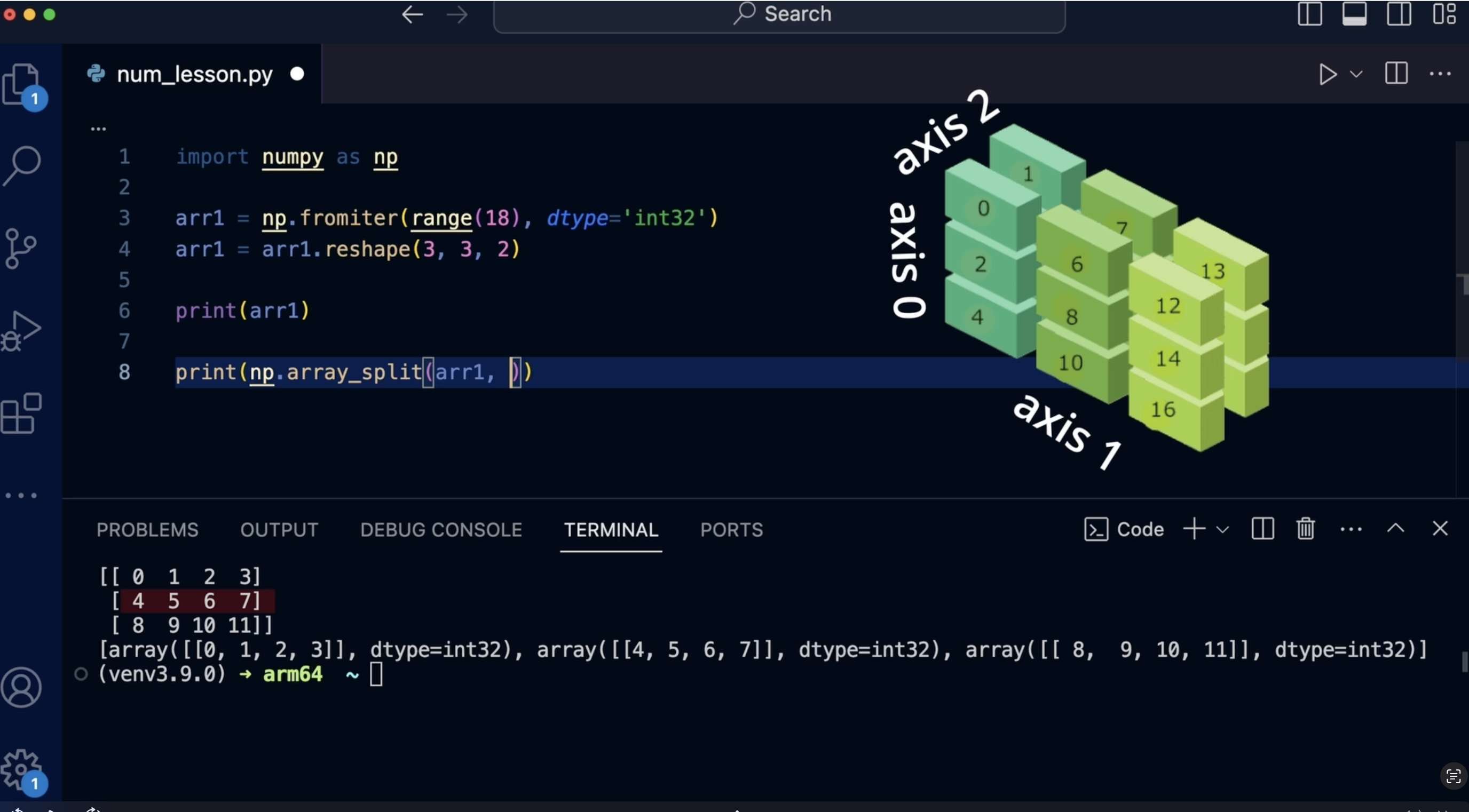
12. Advanced Array Operations and Splitting Techniques: I will remove the necessary
parts and create new arrays. I will show another
way to do it. The FramterFunction in the
Nabi library is used to create a one dimensional
array based on an iterator. It takes a sequence
of values from the iterator and converts
them into an array. We pass an iterator
or a sequence of values from which we
will create an array. You can also specify
the D type parameter, which is the data type to which the values of the iterator
need to be converted. There is an optional
parameter count, which is the number of us
to take from the iterator. By default, this
parameter is minus one, which means taking all values. In our example, we create the first array of four
numbers using range. In the second array,
we also use range, specifying that four numbers are taken from the range
four to eight, so they are difference from the numbers in
the first array. Let me introduce you
column stack function. The column stack function
in the Napi library is used for horizontal concatenation
or sticking of array. We pass atuple of arrays as the columns of array that
we want to concatenate. Let's print it out
to see what we got. It's a convenient tool
for creating array, especially when you
want to combine data from multiple
arrays as columns, and we see our arrays. The first two were
generated as examples, and the third one is the
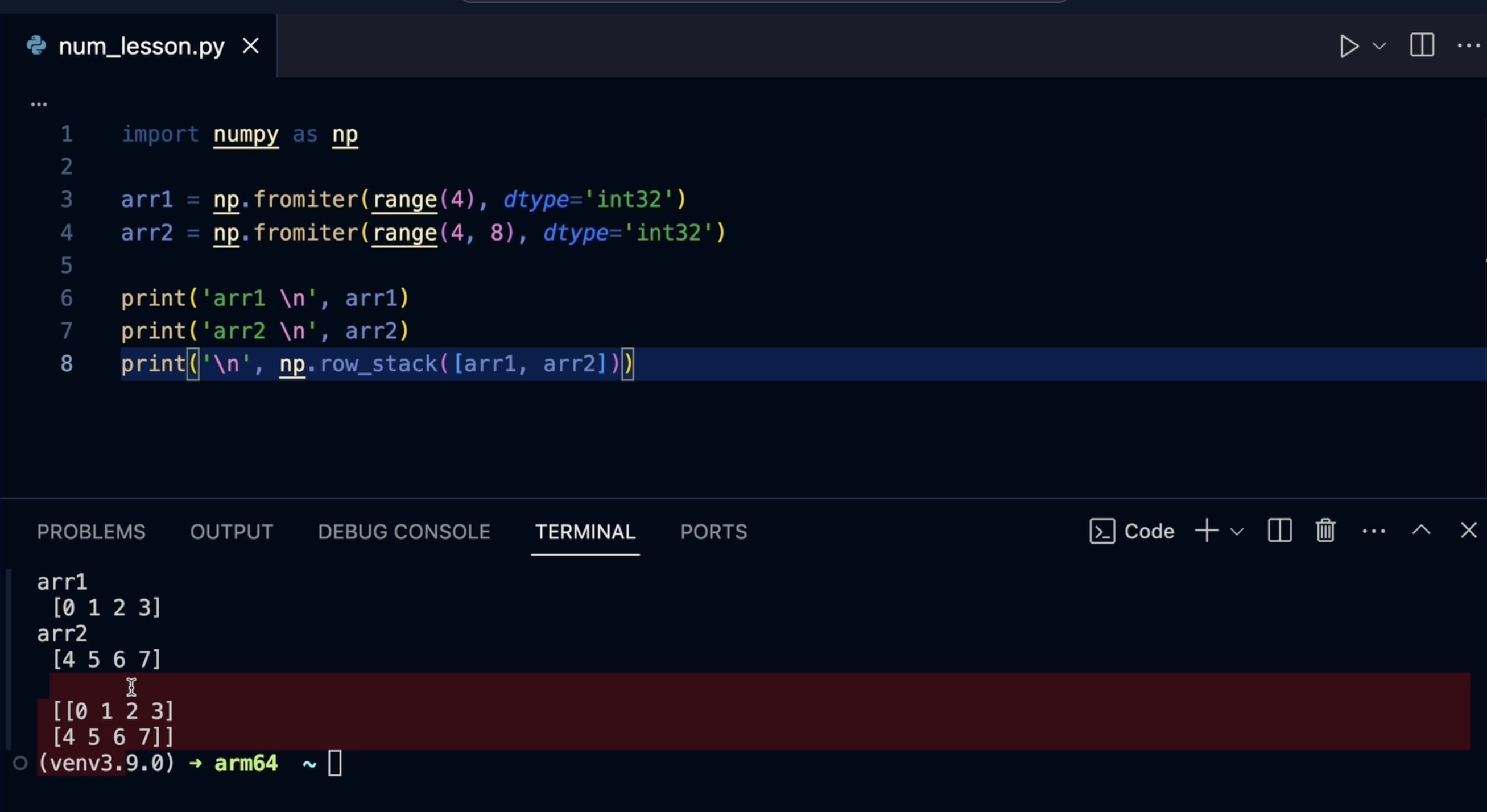
sum of our two arrays. There is a similar
function rows tech, but it's for combining data
from multiple arrays as rows. In this case, the result is the same as if we used
the Vtach function. I will add an empty line to separate the
arrays for clarity. I also can use np dot R. It's an instance of the
R class object in Napi. It acts as a convenient
array concatenation tool allowing you to quickly create and merge rays
along axis zero by rows. I also can use the C. It's an instance of the C
class object in Nampi. It's a convenient tool for
column wise concatenation, meaning it merges array
along axis one by columns. I'm showing you this so that you know the possibilities
of concatenation. You can choose what
works best for you. I will remove unnecessary
parts to avoid clutter and generate an
array of ten numbers 0-9. The H split function is used for horizontally splitting an
array into sub arrays. It divides the array
into equal with sections along the
horizontal axis. It takes the original array. We want to split the
first parameter, and the second parameter is how many parts we want
to split the array into. If I try to split the array
into three parts when its length is not divisible by three, I will get an error. However, in our case, if I specify five, the array will be split
evenly into five sub arrays. We can also split the array into two equal parts. Its
length allows it. V split is a function in umpi used to split an array
vertically along rows. It divides a given array into multiple sub arrays
along axis zero. Since we are splitting the array vertically, we got an error. We cannot split one
dimensional array by columns. I will generate a slightly
larger array and use the reshape function to form a new two dimensional
shape of the array. Let's run it. There is an error because we cannot
split this array into two, but we can split it into three. This function is especially
useful when you need to separate a matrix into
smaller row is sections. Let me increase the array for the next example and make
it three dimensional. If we need to split the array, not just horizontally
or vertically because there can be more dimensions if the array is
multidimensional. The axis can be not
only zero or one, we can use the ray
split function. It splits the array into the
specified number of parts. The second argument is
the number of parts, which is two in our case. And the third
parameter is the axis. In our case, I specified
axis equals two. So it's split along
the third dimension. Specifying axis equals to Numbi function means we are operating along
the third dimension, depth of a three
dimensional array. The split function in Numbi allows spliting along
the third dimension. Even if the number of parts
does not divide evenly, it distributes
elements as evenly as possible among the
resulting sub arrays. But if that's not possible, it will create parts with
different numbers of elements. In our case, we will
get three sub arrays. Two will contain data, and the third will be empty. We can also experiment
and split along axis sequels one or
axis sequels zero. I suggest pausing here
and experimenting. Practice a little.
Now, for example, I will create the simplest list and the simplest
array in Python. Operations between lists and rays have different
natural behaviors. In the case of lists, the plus operation
performs concatenation. That means joining
two lists into one, but it doesn't perform
arithmetic addition of elements. In the case of numb arrays, the plus operation performs
element wise addition, meaning it adds corresponding
elements of the array. Look at the difference
between two print function. One, adding lists and
one adding array. We can also perform element
wise multiplication of two arrays of the same size. Or multiply each
element by number. If I specify this
operation to a list, it will repeat the entire list
at the specified number of times rather than performing element wise multiplication
like an umpire arrays. When you perform the
minus operation, each element in the array changes its sign
to the opposite. The result of this
operation will be a new array where each element of the
array is divided by one. Instead of one, it
can be any number. This operation returns to the remainder of each
element when divided by two, effectively identifying even and odd numbers
in the array. If you subtract a list
from an array Numbi, the list will be
converted to an array, and element Y subtraction
will be performed. However, you cannot subtract list from a list. You
will get an error. Multiplying a list by list
will also result in an error. Now I want to introduce
another concept, and for that, I will create two
dimensional array and 11 dimensional array. There is also the
concept of broadcasting. Array broadcasting is a
mechanism in Napi that allows performing operations on array of different shapes
or dimensions. If two rays have different
number of dimensions, new dimensions are automatically
added to the array with fewer dimensions until
their size are compatible. In other words, if we have the same number of elements
in each row of array, when we add two rays, the smaller array
is concatenated row wise with the rows
of the second array. For this example, I will
create a simplest array again. Let's get acquainted with
the combined operator. When we perform the
addition operation, we can do it more succinctly. In this example, we're adding the number five
to each element of the array and updating its initial value to
the sum with five. This operation is equivalent
to using this notation, but it's done directly in the array without
creating a new object. It's useful because it allows efficiently increasing
or decreasing the values of all elements of the array without needing
to create a new one. This can also be applied to other mathematical
operations.
13. Loading, Saving, and Searching in NumPy: Imagine we have the text file from which we want to load data. The gen from TXT method
is designed to read data from a text file and automatically
determine data types. It's a powerful tool
for working with data in formats like CSV, TSV, and other text formats. Now, let's load data
from the file data TXT. Where the data is
separated by commas, then we specify the
limiter equals to coma. This method can
automatically handle missing values and other
data peculiarities. Let's output this data
in an ampiray if we use Jen from Txt to read numbers separated by
commas from a text file, the output in the console
will typically be a Numpi array with the
values loaded from the file. The values will be
displayed as an array where each number is an
element in the array. The same function in the
Numpi library is used to save numpi arrays in
binary format in a file. This allows saving array
data so that it can be used later without the need to reloading or recomputation. If we open the file created
with the saved array, we will not see
anything useful for us. However, the load
function is used to load such saved arrays back
into the program's memory. It allows accessing the data of the array that was saved
using the safe function. These functions are very useful for working with
large amounts of data and further processing them without the need
for a computation. The savetixt function
in the Napi library is used to save Nampi arrays
in text format in a file. This allows saving array data in a format that is convenient
for reading and editing. For example, I will
choose the CSV format, but you can specify extensions
like Tixt, CSV or data. These are common extensions usually used for storing
data in text format. However, SaptixT
can actually save data in any text file with
any extensions you want. We can see that our file appeared in the
project directory. Now let's load it. The od text function
is used to load data from a text file
into an AmpiRray. It allows accessing data that was saved using the
save Tixt function. This is very similar
to the mechanism we discussed earlier where we
used save and then load. But that format wasn't user
friendly or readable for us. Here, however, we can already see the file and
it saved contents. These two functions are very
useful for working with data in a format
understandable to humans. They allow easily saving
and loading data without the need to understand the internal structure
of Numprays. For the next example,
let me create U Suppose we have a two dimensional array
representing some data. Well, let it be temperature
in different regions, and we want to find
the position of all elements that exceed
a certain threshold. I define a variable threshold
and the value of 30. This is the value about which we want to find
elements in the array. How can we do this in Nam Pi? There is a function that
is particularly useful for finding the position of elements that satisfy given condition, and this is the
arc ware function. Our condition returns
the indices of the element that are true in
the boolean array because this expression creates
a boolean array where each element is true if it's greater than
30 and falls otherwise. I print the original data array to provide context
for the position of the elements and then
print the indices. These indices are returned
as two dimensional array, where each row represents the
coordinates of an element, the row index, and the column index in
the original array. The output shows that the
elements greater than 30 are located at the following position
in the data array, Row one, column two, element 35. Row two column zero, element 40. Row two column one, element 45, and so on. In this example, I demonstrated how Arcbar
function can be used to locate the position
of elements and numpy array that meet
a specific condition. Congratulations. We
finished this crash course. I hope you found it
interesting and not too boring and that you
found this lesson useful. Once again, I want to emphasize that practice is
the most important thing. I highly recommend pausing
after each lesson and experimenting or
repeating something manually because theory is good, but you will not learn
without practice. The best way to learn is
through your own practice. Thank you for your attention and keep coding, keep learning.
 Olha Al, Software engineer