Transcripts
1. Intro: Hi, guys. Are you tired
of slow data processing? Do you struggle
with large datasets that push your system
to its limits? If you work with data and need speed efficiency
and scalability, this course is exactly
what you need. Let's get acquainted with
the Pollard's library, and we will compare it with
the ever popular Pandas. If you are tired of waiting for large amounts of data to
load and process in Pandas, this tutorial is for you because this library is
set to replace Pandas, but will it really
be able to do that? Unlike Pandas, polars is
designed to easily handle large datasets using advanced parallel processing
and lazy evaluation. That's what we will
explore in this session. We will cover the
basic principles of how polars operates, discuss its advantages
and disadvantages, and compare it with Pandas in terms of performance
and usability. We will also go through the main functions for working with data using principal examples to illustrate these concepts. You'll discover how polars
outperforms Pandas. When working with datasets
over 100 million rows, you'll learn how to
process data in chunks, allowing you to work efficiently without running out of memory. We'll explore data visualization and polars, and
most importantly, you will understand lazy mode, the secret behind polars
and matched speed. By the end of this tutorial, you will have a solid
understanding of how to use polars for
your data analysis needs and be able to decide whether it's the right tool
for your project or not. So ready to take your skills to the next level,
let's dive in.
2. Introduction to Polars: Key Differences from Pandas and Why It’s Faster: Hi, guys, let's get acquainted
with the polars library, and we will compare it with
the ever popular Pandas. Polars is a fast and
efficient data frame library designed for working
with large datasets. It is built with
performance in mind, utilizing multi threading and parallel processing to handle data manipulation tasks quickly. Polars is implemented in RST, which allows it to
offer superior speed compared to other data frame
libraries like Pandas. The library supports
operations such as filtering, aggregation, and
transformation of data, and it's particularly useful
for data analysts and data scientists who need to work with large volumes
of data efficiently. With both a Pattern
and Rust API, polars is accessible and powerful for modern data
processing workflows. As I said before, this library
provides a wide range of functions for data manipulation, aggregation, and transformation. But in my opinion, its main
feature is lazy evaluation. What is lazy evaluation? As evaluation is a computational
strategy that delays the execution of an operation until its result is
actually needed. In the context of polars, this means that data
manipulation operations aren't executed immediately
when they are defined. Instead, they are recorded as a series of steps to
be executed later. This approach allows polars to optimize the entire
sequence of operations, reducing the overall computational
workload and improving performance by only executing necessary calculations
at the end. Another important feature is
multi threaded processing. One of the key advantages
of polars its ability to process data using multiple
threads at the same time. This means that
instead of performing tasks one after
another sequentially, polars can split
the workload into smaller parts and run them simultaneously across
multiple CPU course. They significantly speed
up data operations, especially when working
with large datasets. Polars achieves the efficiency because it's built with rust, a programming
language designed for high performance and
safe memory management. Rust makes it easier to work
with parallel computing, meaning that polars can
fully utilize the power of modern computers with
multi core processors. Another powerful feature in polars is its ability
to memory map data. It means that instead of loading an entire large
dataset into Rum, which could slow
down your computer or even cause it to crash, polars can read and process only the parts that are
needed at the moment. For example, if you
are working with massive CSV or Parki file, polars doesn't need to load
the whole file into memory. Instead, it accesses the data directly from the
file as needed, making the process much faster
and more memory efficient. These features make polars an excellent choice for
working with big data. As it helps analysts and researchers handle
large datasets quickly and effectively without requiring high end hardware, polars is built on
top of apache arrow, a data format designed to make data storage and transfer
faster and more efficient. Think of arrow as a
high optimized way to organize and structure
data so that it can be processed quickly by different systems because
arrow is used by polars, it allows polars to share
data seamlessly with other tools and systems
that also use arrow. Example, if you're working in polars and want to
pass your data to different system like a
Machine Learning tool or another data
analysis library, AR makes that data transfer
happen smoothly and efficiently without needing to convert data into a
different format, which can be slow and costly. Another feature that makes
polars user friendly, it's ponds like API. Pandas is one of the
most popular tools for data analysis in Python, and many data analysts and scientists are already
familiar with how it works. Polars was designed to feel
familiar to Pandas users. So if you already know Pandas, you can start using polars without needing to learn
everything from scratch. However, while the
API look familiar, polars have the added
performance advantage of being faster and
more efficient, especially when dealing
with large datasets. So if you are
coming from Pandas, you can benefit from the
same easy to use syntax, but enjoy the speed and
memory efficiency of polars. Even though polars has
many great features, there are some
limitation to consider. It's important to keep in
mind that like any tool, it may not be the best
fit for every situation. We will go into more detail about these drawbacks later on. But for now, let's take a look
at some of the challenges. One potential disadvantage
is that polars is relatively new compared to more established
libraries like Pandas. Since it's still growing, there may be fewer resources
available such as tutorials, community support,
or documentation, which could make it harder
for beginners to get started. Also, since it's new, there may be fewer
examples of how companies are using it in real world,
large scale projects. Because polars is not
as widely adopted yet, there is limited
information about how many companies are using it in production
environment, the real world systems where companies run
their operations. Most companies that
use polars might not publicly share details about how it fits into
their workflows. So it's harder to
know how well it performs under very large
or complex workloads. However, some
companies are starting to use polars for their
data processing tasks, and you might see examples
of this in the industry. As the library matures, its adoption will
likely grow and more companies will start
sharing their experiences. So let's get started.
3. Installing Polars, Loading DataFrames, and Accessing Columns Efficiently: Here's the command to
install the library. Let's get started. I will open my terminal since I'm
used to working with it. First, I will activate
my virtual environment. If you're not familiar
with virtual environments, I strongly recommend checking
out my video on how to manage virtual environments and how they can make
your life easier. But if you don't know what
a virtual environment is, you can run the command
directly in the terminal. Right now, knowing
how to work with virtual environment
is not priority. After activating my environment, I can run my Jupiter
notebook right from the terminal by executing the
command Jupiter notebook. If you use Anaconda after
starting Jupiter Notebook, you can install this
library directly inside Jupiter by running
the following command. As you can see, I already
have the library installed, so we can start working. First, I will import all the necessary libraries
that we will be working with. I'm importing the Numbi
library because we'll need it. For those who aren't
familiar with it, Nampi is a powerful
Python library used for numerical computing. In my profile, you can find
a utorial on this library. Then I will check the
version of polars. I've downloaded a huge dataset
over 1 gigabyte in size, and now I'm going to import it using the Read CSV
function in polars. It takes a little time to load then using the
shape function, which you may have
heard from Pandas, we can check the
dimensions of our dataset. If you're not familiar with it, the shape function and
polars returns the double representing the number of rows and columns
in the data frame. This function is
useful for quickly understanding the
size of your dataset. And here we can see that the dataset contains more
than 130 million rows. Another useful function for quickly understanding
a data frame without loading all the
data in the head function. By default, it displays
the first five rows. As we can see, the appearance of the data frame in polars is slightly different from what we observed when loading
data with Pandas. The first noticeable
difference in the data type information
displayed for each column. Using the two Pandas
function in polars, we can convert Polars data
frame into Pandas dataframe. This is particularly useful when you need to leverage Pandas specific functionality
or integrate with libraries that only
support Panda's dataframes. The two Pandas method ensures a smooth transition
between polars and Pandas, allowing you to
take advantage of both libraries within
the same workflow. If you don't want to download large datasets onto
your computer, you can use publicly
available datasets on Github. To do this, find a large
dataset on GitHub. Go to the row tub and
copy the direct link. Use the reads as we function
in polars to load it. Like before, it takes a
little time to process. But eventually, we
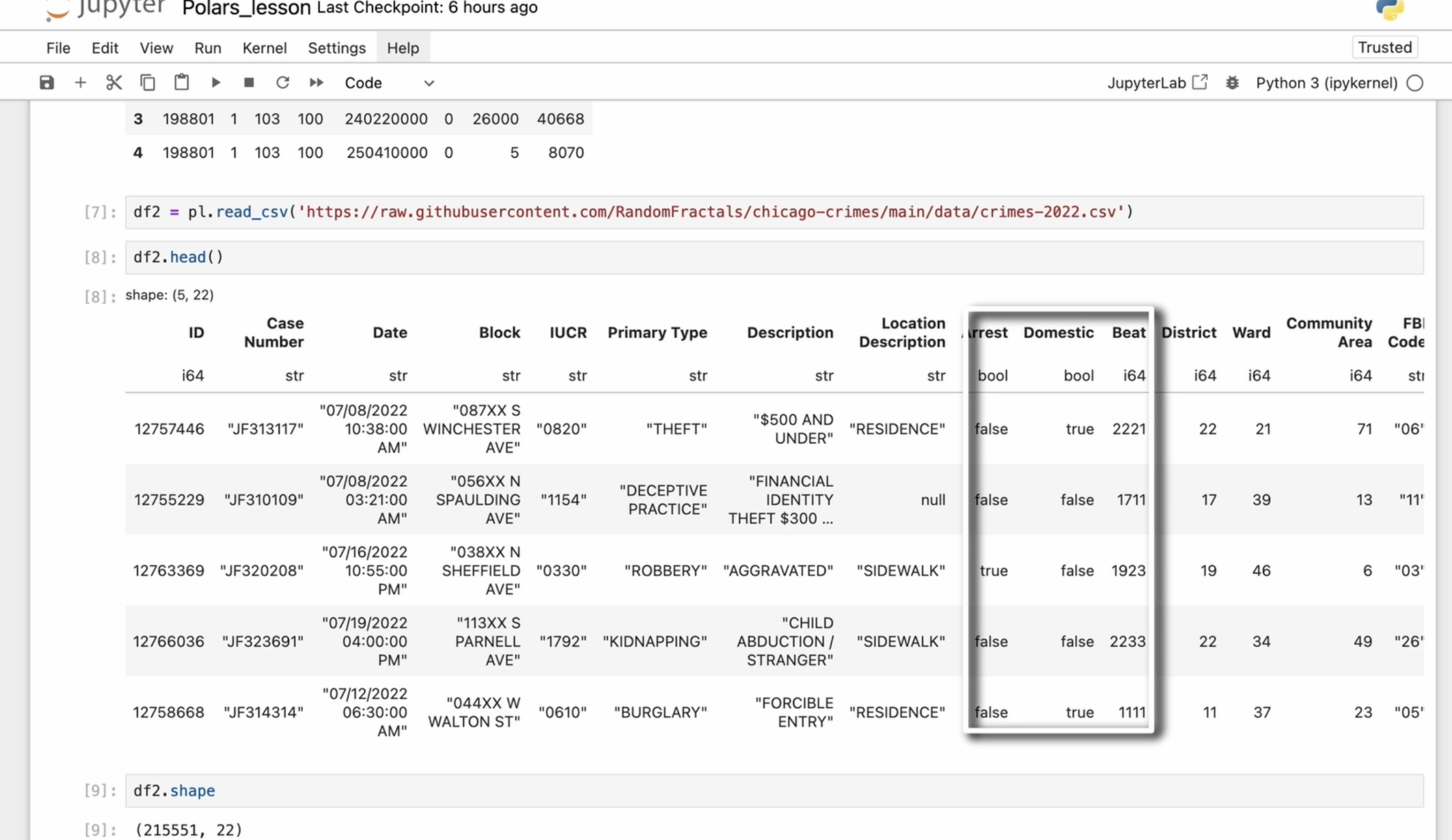
can see the data. For today's example,
we are working with the Chicago crime
data set of for 2022. We can also check
the column types, and we can see that it
contains 2,525,551 rows, quite large but not
too overwhelming. To avoid confusion with the first data frame
we loaded earlier, I'll rename this new data frame. I will still use the
first data frame later, but for now, we will work
with this second one, which was loaded from Github. I will reload it all cells, just like in Pandas. In polars, a series is
one dimensional array like structure that represents a single column of a data frame. It can contain
homogeneous data types, such as integers, floats,
strings, buoyans. Series are the building blocks
of data frames and polars. They allow us to perform various data manipulation
and analysis operation, such as filtering,
transformation, and aggregation. Each series has an associated
name and data type, making it easy to reference
within the data frame. We can extract a series from a data frame
in several ways. The first one using
the column name. The most straightforward way is accessing the column by name. To avoid loading the entire
series in large datasets, I will use the head function to display only the
first four rows. The second one using
GAD column function. This approach has performance
and flexibility advantages over direct column access. For me, the main reason to use Get column function is
its error handling. If you try to retrieve
a non existing column, pullers immediately
raises an error. This provides instant feedback if there is a typo
in the column name. In contrast, accessing
a column by name may either silently return
non or raise a key error, which can make debugging harder. The third way is
the select method. It creates a new data frame containing only the
specified column. However, even if it
contains just one column, the result is still
a data frame. To work directly with a series, we need to convert it
using two series function. The select method
in polars returns a new data frame even if we are selecting only
a single column. This means that if I create a one variable and assign
this result to it, it's not just a single column, but the polars data frame
containing one column. So if I check the
D type of a one, also I remove two series method. It might result in an error. As D type is typically an attribute of series,
not a data frame. And here we are,
we have an error. If I again use two
series method, as one is no longer
a data frame, body polar series and D type attribute will return the data type
of district column. Let's print it out.
In the first case, we can see that print as one, displacing the value of the
district column as a series. Here we can see the shape, the data type, and the values. The second case displaces the district column inside
the data frame format, showing the column
name and its data.
4. Data Manipulation in Polars: Arithmetic Operations, Column Management, and Filtering Techniques: In polars, we can perform
arithmetic operations on series or columns using
standard Python operations. For example, we
can use addition. If we want to add
ten to a series, we can see that each number
in the resulting series has increased by exactly ten compared to the number
in the original series. Here I print the original series and we can see the result. Age value increases by ten. Multiplication.
Multiplying a series by two doubles each value. Here I compare to
the original series, and we can see that
each value is doubled. Subtracting 20 decreases
each value by 20. Let's go on with
aggregation methods. Polars provide built in methods for aggregations,
such as sum. The sum method in polars is
used to calculate the sum of all elements in a series or
a column in a data frame. When applied to a column
containing integer values, it returns to the total
sum of those values. The mean method in
polars calculates the average of all elements
in series or column. In our example, it computes the arithmetic mean of all
integers values in our series. We can also use
comparison operators in polars to create
Boolean series. In polars, comparison
operators allow you to compare values in a
column with other values, and the result is
a boolean series. A boolean series is a sequence
of true or false values, which you can use to filter, analyze, or
manipulate your data. Here's how the eparators work. In this case, we create a new series containing
Boolean values. The operation compares
each value in the column with 20
and returns a series of the same length at
the original column where each element is
either true or false. Also in polars, we can use
the greater than method. At first time it
returned only false, so I changed the
comparison value to 30. This method is used to compare a column with a specific value, similar to using the greater than operator
that we used earlier. The greater than method is a built in function that performs, yes, the same operation, but allows for more flexibility. It can be useful when
working with methods that require function calls
instead of operators. In some cases, it may
be preferred when using method chaining or working with custom expressions
in a query. So the first case we can use when checking values
in a data frame. The greater than method that
we used in the second case, we can use when we need
function based processing, such as method chaining or compatibility with
certain query structures. In most cases, both approaches
achieve the same result. This is useful for
filtering or analyzing data where you want to
focus on values that meet a specific
condition like finding records with higher sales
than a certain target. I between this operator checks if a value falls within a
specific range of numbers. For example, using is 20-30 will return
true for all values. In the column that are
between ten and TG, including ten and TJ and falls. For those that are
outside of this range, this is particularly helpful when you need to filter data or create conditions that check if values lie within
a specific range, like age 18-65 or
prices $10-100. In polars, adding
a new column to a data frame is done using
with columns method. It's important to know that polars data frame are immutable, meaning that the
original data frame doesn't change when
you add a new column. Instead, this method creates and returns a new data frame
with a new column added, leaving the original
data frame unchanged. So we use with columns method. It tells polars to add new
columns to our data frame. To add a constant
value to a new column, we use lead function. This function creates a
literal or fixed value that will be assigned to
every row in the new column. Example, if we use t one, it means every row in the new column will
have the value one. After creating new column, you can give it a name using AS. In our case, I call
it new column. This is how you specify what the new column will be
called in the data frame. After executing these steps, we create a new data
frame based on data frame two with a new column
named new column added. The new column contains the
value one for all rows. And as expected, the
original data frame remains unchanged. If you want to delete
column from a data frame, you can use that drop method. This method allows you
to remove a column by providing its name
as the argument. You simply need to tell polars which column you want to remove by specifying
the column's name. It's important to know that polars data frames
are immutable, meaning that the drop method doesn't modify the original
data frame directly. Instead, it creates
a new data frame with the column removed. This is done to ensure that the original data
remains unchanged. Since the original data
frame doesn't change, if you want to keep the
modified data frame, the one without the
dropped column, you need to reassign
the result back to the original variable or
store it in a new variable. Without doing this, the
original data frame will remain unchanged. Now let's look at filtering a polar series based
on certain conditions. For example, here we are filtering to keep only
the even numbers. The condition checks
for even numbers, and the filter method keeps only those elements where the condition evaluates to true. This is really useful, as you can adjust the condition and sign the filter to filter the series based on
different criteria. For instance, I filtered
all values greater than 20. If I change it to 30, the condition
becomes more clear. Let me quickly update that and restart the cell for
the next example. Now, let's create two series. Probably it's better to
use just name series. I removed the print operator because Jupiter notebook
render it great. And the second series is just slightly
different from the first. Now let's concatenate them. When working with pullers, the concatenation of series
depends on the data type. If you concatenate two string type series using
the plus operator, the operation performs element wise concatenation
of the strings. This means that each
element in the first series is concatenate with
the corresponding element in the second series. Since both series
are the string type, the plus operator
concatenates the strings. However, when series of
different types are involved, polars will automatically
cost the series to compatible data type before
performing the operation. Here, polars automatically
converts the integers into strings before
performing the concatenation. If you concatenate two
integers type series using the plus operator, the operation will perform
element wise addition of these integers, not
string concatenation. As a result, the series will
contain summed integers.
5. Mastering DataFrames in Polars: Slicing, Descriptive Statistics, and Advanced Data Exploration: Let's quickly review how
to access rows and polars. In polars, you can access rows using indexing and slicing, similar to how it works in other data manipulation
libraries like Pandas. However, there are some key
differences in how polars handles rows due to its
columnar data structure. You can access rows
using indexing, but polars returns
a new data frame instead of single row object. When you access a specific
row using an index, polars returns it as a
new data frame rather than as a single tuple or
individual row object. This is different from Pandas, where accessing row returns a series one dimensional object. Since polars is optimized for working with columns
rather than rows, this behavior ensures
that data remains consistent and efficient
when performing operations. You can also extract multiple
rows using slice notation, which works similarly to how you slice lists or ray in Python. This allows you to
retrieve a range of rows efficiently without changing
the data frame structure. Unlike Pandas, polars doesn't
use an explicit row index. Instead, rows are identified
by their position, making it more efficient when working with large datasets. This columnar approach
helps polars perform data operations much faster than traditional role
based indexing methods. The described
method in polars is a powerful tool used to generate descriptive
statistics for a data frame. Descriptive statistics helps you summarize and understand the
key features of your data, allowing you to quickly get an overview of its
characteristics. Here we can see what the
described method provides. Count shows the number of non
null values in each column. It helps you understand how
much data is available for each variable and whether
there are any missing values. The mean or average of
each numerical column, it gives you an idea of the
central tendency of the data. What value is the most
typical for that column? The standard deviation tells you how spread out the
data around the mean. A small standard deviation means the values are
close to the mean, while a large standard deviation means the values are
more spread out. Depending on the data, pollers may also provide
other statistics, which gives more insights into the distribution of
values in each column. The described
method is great for quickly gaining insight
into your data. It helps you identify patterns and understand the general
behavior of the data, detect outliers or values that are usually
far from the mean, get a sense of how much
variation exists in the dataset, which can help with
making decisions about how to clean or
process the data further. The estimated size method
in polars is used to estimate how much memory a data frame will
use in your system. It gives you an approximate
size of data frame, so you can understand
how much space it's taking up in your memory. When you call estimated
size on a data frame, it calculates the memory usage of the data frame in megabytes. This is useful when
you're working with large datasets and want to ensure your system has enough memory to process
them efficiently. Instead of loading the
entire data frame and seeing how much space
it uses in memory, which can be slow
or inefficient, you can get a quick estimate. The duplicated method in
polars is used to identify duplicate rows within a data
frame based on all columns. It returns able and series, indicating whether each row is a duplicate of a previous row. To get only the duplicated rows, we can filter the data. This will remove all
non duplicated rows, leaving only the duplicates
in the resulting data frame. As we can see, there are no
duplicates in this case. These empty method
and polars is used to check whether a data frame
contains any data or not. Essentially, it helps you determine if the
data frame is empty, meaning it has no rows
or data inside it. For example, you could have a data frame with column names, but no data in the rows. This would be considered empty. When you use is empty method, it checks if the data
frame has any rows. If the data frame has no rows, it will return true, indicating that the
data frame is empty. If the data frame has
one or more rows, it will return false, meaning the data
frame is not empty. This method is especially
useful in situations where you might want to perform some operations on a data frame, but only if it contains data. For example, before performing a complex calculation
or data transformation, you may want to make sure the data frame actually
has data to work with. This can prevent errors or unnecessary computations
on an empty dataset. This unique method in
polars is used to check whether the values in a
particular column are unique. When you call is unique method on a column in a
polars data frame, it checks whether all the values in that column are unique. The method will return
true if every value in the column is unique and falls if any values
are repeated. It helps in cleaning
or validating data before performing
tasks like analysis, merging datasets, or
creating indexes. Here I used the filter again to get unique values instead
of just or false. Ports also provides
unique method, which counts the number of unique values in a
series or data frame. It returns an integer representing the count
of unique values. When applied to a column, and unique returns the total count of distinct
values of that column. If used on a data frame, it typically counts
unique values for each column separately. And unique method is
helpful when analyzing data to understand its
diversity or spread. It can be used to detect
duplicate values. For example, checking how
many different customers IDs, product names or user
emails exist in a dataset. It helps with data validation, ensuring that a
column meant to have unique values doesn't contain
unexpected duplicates. The null count method and
polars is used to count the number of missing values in a column or an
entire data frame. When applied to a column, it returns the total number of null values in that column. If I use it on a data frame, it typically counts null values for each column separately. Missing values can cause
issues in calculations. So knowing how many null values exist helps decide
how to handle them. If a column that should always
have data has null values, it may indicate
data entry errors. Many machine learning models cannot handle missing
data directly. So counting null values is the first step in deciding
how to fill or remove them. The count method in polars is
used to count the number of non null values in a column
or an entire dataframe. It helps you quickly determine how many actual non missing
values exist in your dataset. When I apply this
method to column, it returns the total number of non null values
in that column. If I use it on a data frame, it typically counts
the non null values for each column separately. It helps determine
how much usable data is available in each column. By comparing count null values with a total number of rows, you can see how many
missing values exist. Many data processing steps
require non null values. So knowing how many
valid entries are present helps with data
cleaning and processing. The mean horizontal method in
polars is used to calculate the mean or average values across horizontal
rows of a data frame. It computes the mean for
each row individually, treating each row as a
separate sequence of values. This method is useful for summarizing data and
gaining insights into the distribution and characteristics of
values within a dataset. To find the minimum or maximum
values in a dataframe, you can use methods
like mean and max. The mean function returns at the minimum value across all numerical columns
in the data frame. The max function gets the maximum values across
all numerical columns. These functions work not
only with numerical data, but also with other types of data such as strings or dates. The product function in polars is used to calculate
the product of all values in a column or series or multiple
columns in a data frame. This means it multiplies all the values together
and returns the result. When applied to a column, it returns a single number representing the product of
all values in that column. For data frame, it calculates the product for each
numerical column separately. It's very useful for
mathematical calculations, financial analysis
and data validation. If you want to estimate the
spread or squared deviation of values from their mean
in each numerical column, you can use the var function. It measures how much on average values in a column
deviate from the mean. It's commonly used in
statistical analysis to understand the distribution
and variability of data. The SDD function computes the standard deviation of values in each column
of a data frame. This function returns a series containing the standard
deviation for each column. A low standard deviation means that values are
close to the mean, while a high standard
deviation indicates that the values are spread
out across a wide range.
6. Exploring Polars DataFrame Methods: Flags, Schema, Column Operations, and Data Conversion Techniques: The flag function
and polars returns a dictionary of flags for each
column in the data frame. Each flag is presented
a boolean value indicating whether the flag is set for that column or not. For example, I see
sorted flags here, but if I want to check
whether a column is unique, I can use this unique function. This unique function
returns a boolean value. True if all the values in the specified
columns are unique, no duplicates and false if there are any
duplicate values. And here I check whether the distinct column in my data frame contains
only unique values or not. In the first case, I checked for the presence of unique
values in the column, whether they exists at all. And then we found out whether the column consists
entirely of unique values. And as we can see, there
are no unique values, and the column is not marked
with the unique flag. To retrieve the list of column
names in the data frame, you can use the columns method. It returns a list of strings where each string
is the name of column. This is useful for quickly checking the structure
of the data frame and understanding
which columns are available for analysis
or processing. The schema of a data frame
refers to its structure, specifically the column
names and their data types. In polars understanding,
the schema is important because it helps you know what kind of data
you're working with. The schema includes the names of all columns in
the data frame, and this helps you quickly
see what data is available. Each column in the data
frame has a data type, and knowing the data types
is also important because some operations only work
on specific types of data. So schema helps check if the data is in the
correct format before performing operations. Some operations might fall if the data types is incorrect. So checking the schema
beforehand can prevent errors. The width method
in polars is used to find how many columns are
presented in a data frame. This is useful when working
with large datasets. Where manual counting
columns is impractical. It helps quickly check how many different data
fields exist in your dataset. It also can help when working
with dynamic datasets. Knowing the number of
columns can help with tasks like looping through columns
or selecting specific ones. The glimpse method in polars is used to preview a summary
of your data frame, giving you a quick look
at the data structure. It's helpful when you
want to understand the general layout of your data without having to display
the entire dataset, especially when working
with large datasets. Glimse method provides a
compact overview of data frame, including column names,
data types of each column, a preview of the first few
values in each column. This method doesn't show
the entire dataset, but instead offers
a quick snapshot, so you can understand the
data structure at a glance. It helps to quickly check
what data is available, what the columns are,
and the types of data you're working with
without displaying everything. It also helps you avoid
overwhelming yourself with large amounts of data by only showing a small
summarized portion. You can also spot
potential issues like unexpected data types, missing values or
inconsistencies in column names during
this quick review. The N chunks method in
polars is used to find out how many chunks a data frame
is divided into internally. In polars, data can be split into chunks for more
efficient processing, especially when working with large datasets that do not
fit into memory all at once. A chunk is a smaller portion
of the entire data frame. Polars often divides
large datasets into chunks to handle them
more effectively in memory. Each chunk can be
processed separately, allowing polars to
work with datasets that are too large to fit
entirely into memory at once. This is part of Polar's efficient memory
management system. When you use the
N chunks method, it returns the number
of chunks that our data frame has been
split into for processing. This can be useful for
understand how polars is managing the memory
and data distribution for your specific data frame. In some cases, understanding the chunking of data helps you monitor and debug how polars is handling
data in your program. If a data frame has a
large number of chunks, operations might
be less efficient compared to when the data is
stored in a single chunk. Understanding chunks is key when working with
large datasets. The two arrow function
and polars is used to convert a polars data frame
into a Pache arrow table. This is useful for
data interoperability because apache arrow is widely used format for efficient data exchange between different data
processing systems. Apache arrow is a
columnar memory format designed for fast
data processing. It allows different
data processing tools like Pandas or Spark to share data
efficiently without needing to copy or convert
it multiple times. When you use two arrow function, Poller's transforms its
internal data format into a patch arrow table while
keeping the columnar structure. It helps with faster
data sharing, efficient memory usage,
and better compatibility. Polars also provides
the two digT function, which converts a data frame or series into a Python dictionary. Each column in the data
frame becomes a key in the dictionary with
corresponding values, forming a list for that key. We also have two dicts method. In polars, it converts a data frame into a
list of dictionaries. Many Python functions and libraries work well with
lists of dictionaries. For example, if you need to convert your data
into JSON format, these can be helpful
intermediate step as list of dictionaries are
easily serializable to JSON. If for some reason you need a string representation
of the data frame, you can use the two N
representation method. This is particularly useful for debugging or for scenarios
where you need to generate code that can reproduce that data
frame exactly as it is. Can also use two Napi method, which converts the polars
data frame to NumPy array. This is useful when
you need to leverage Napi's powerful
array manipulation and mathematical functions. Since Napi arrays are highly efficient for
numerical computations, this method is beneficial
when performing operations that are
better handled by Nam Pi. The same I can say about
the two Pandas method. It converts the polars data
frame to Panda's dataframe. This is useful when
you want to use Pandas specific functionality or when working in an
ecosystem where Pandas is primary data
manipulation tool. The two torch method converts a polar data frame
to a Pytorch tensor. This is ideal for preparing data for deep learning
models in PyTorch. However, since I don't have
this library installed, I encounter at and error. We can install this
library with this command, but right now we don't need it, so I leave it as it is.
7. Advanced Data Manipulation in Polars: Grouping, Aggregation, Sorting, and Custom Transformation: Now let's continue with
the group B method. If you have worked
with Pandas before, you're likely familiar
with this method. If not, here's a
quick explanation. The group B method
in polars is used to group a data frame by
one or more columns. In our case, grouping by
the year column means that all rows with the same value in the year column will
be grouped together. Each unique year will
form separate group. However, in our case, we only have one year 2022. Next, we use aggregation. The method and polars
is used to perform aggregate calculations on groups of data within a data frame. We then specify the column, bit, and apply the
count function. This means that for each group, we count the number of
occurrences of the bit column. Essentially, this counts
the number of rows in each group since each row
represents an incident. Then we use the Alias function. To rename the
resulting column from the aggregation to
count incidents. This is done to give the aggregated column
a meaningful name. In theory, we can use this
function to summarize data and understand the
frequency of incidents per year. However, since we only have
one year in our dataset, we only see the count
of incidents for 2022. Now let's consider another
example when I group by year. But instead of using an
aggregation function, I use the L method. The OL method retains all
rows within each group. The seperation is
useful when you need to work with all data
points within each group without performing
any aggregation or transformation that
reduces the dataset. In some cases, when you want to get quick overview
of each group, you can use the first
method instead of all. This is useful when
you want to extract sample data points
from each group or reduce the data frame to one row per group for further
analysis or reporting. I don't have the best
example for this, so let's group by
primary type instead. That makes it clearer. Here we can see the first
row for each group. In our case, the
primary type column. The last method works
almost the same except it returns only the
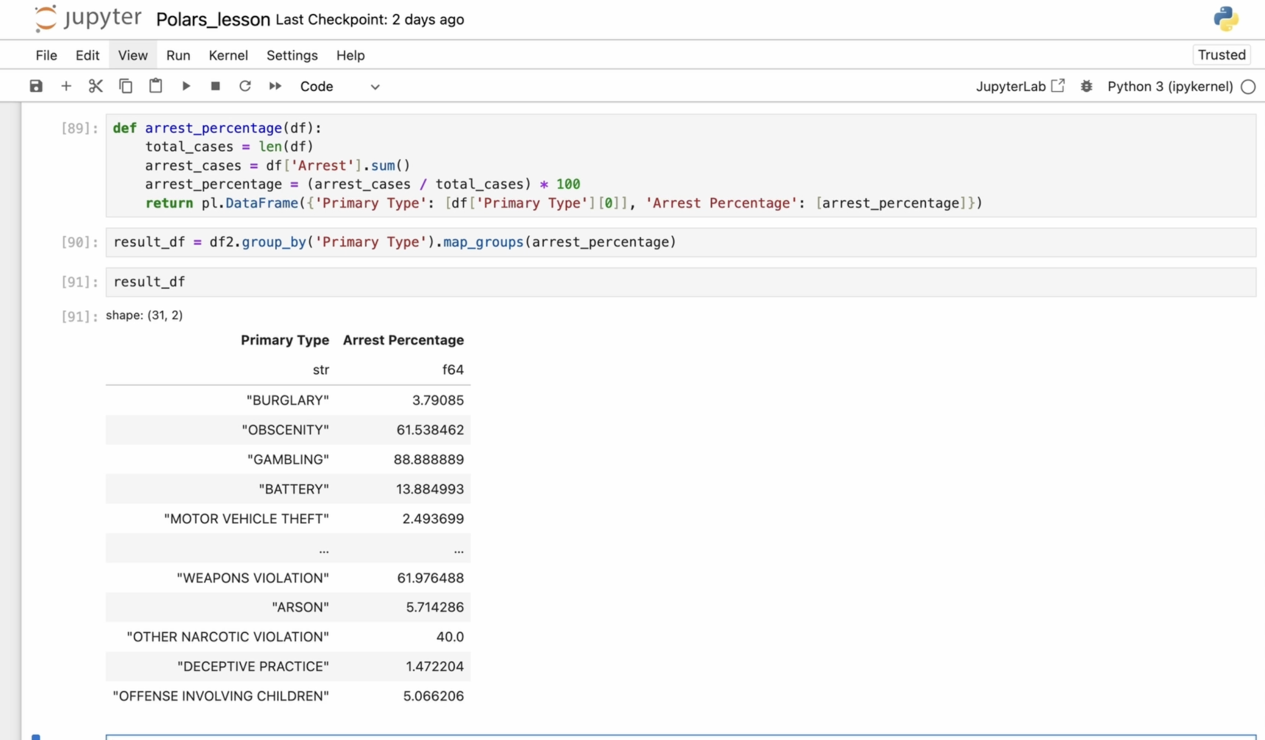
last row for each group. Now I want to define a custom function to calculate
the arrest percentage. First, I get the total number of cases by calculating the
length of the data frame. Then I get the number of arrest cases by summing
the arrest column. Next, I calculate the
arrest percentage by dividing the number of arrest by the total
number of cases. Finally, I return the data
frame with the result. This code groups the
data by primary type and calculates the
arrest percentage for each type of crime. From the result, we
can see which types of crimes have higher or
lower arrest rates. Now that we have created this function, it's
time to use it. A very useful method
for this is nab groups. This method takes the
grouped data as input, applies the custom
function to each group, and then returns
a new data frame with the result of
this operation. In this case, we group
the data frame by the primary type
column and then apply our custom arrest percentage
function to each group. This function
processes each group independently and can perform
any custom logic needed. The result is a new data
frame where each row contains the result of applying the arrest percentage
function to each group. There is also an apply function, which applies a custom
or user defined function in a group by context, however it has been deprecated
and renamed to map groups. So if you see the
apply function in older code, don't get confused. It's just an outdated version. You're probably familiar
with the head function, which allows you to see the first several
rows of a data frame. However, let's consider
another useful function, tail. Let's say I want to see only
the last rows of each group. Using the tail method within
a group allows us to focus on the most recent or last few
entries for each category. This can be useful for examining the most recent cases
in our dataset. In this case, grams, but in other cases, it
could be any type of data. You can also use
the sort function after applying these operations. It allows you to sort the extracted entries
by a specific column, for example, community area for better readability
or further analysis. So what did we do here? We grouped by primary type. We selected the last
row for each group and we sorted the data
by community area. The sequence of operations
helps in analyzing the most recent entries
while improving readability.
8. Advanced Data Operations in Polars: write_csv, Pivot Tables, and Join Strategies: For the next example, I
need two data frames. Joining data frames is a common operation in
data manipulation where rows from two or
more data frames are combined based
on common columns. Polars provides various
types of joins, similar to SQL style joins. Let's print both data frames and start with the inner join. I take my first data frame
and use the join function. Then I specify the
second data frame that I want to join
with the first one. Next, I define the
column to join on. This can be a single column name or a list of column names. In my case, it's name. Finally, I specify
the type of join, which in our case
is an inner join. Sorry for typo. This
means that only rows with matching keys in both data frames will
appear in the result. We see that both Bob and Charlie are present
in both data frames, so we see them in our result. Now let's try a left join. This means that all rows
from the left data frame and only the matching rows from the right data frame
will be in the result. And we can see that all names
and all information from the left data frame appeared in our result and from
the right data frame, in our case, the
second data frame. We can see only two names, Bob and Charlie that are
present in both data frames. For a full drawing, all rows from both data
frames will appear in the result with no values
where there are no matches. And here we can see the
nulls in the result. We also have cross join. It returns all possible
combinations of rows from both data frames,
a cartesian product. Every row from the left is combined with every
row from the right. And to show you all
types of joins, I want to explain
you also semi join. It returns only rows from the left data frame that have matching keys in the
right data frame. You might ask me
what the difference between inner join and semijoin? We got almost the same. Both inner join and semijoin returns rows where there is a match
between two tables, but they have a key difference. Inner join returns all matching
rows from both tables, including columns from both. Semijoin returns
only the rows from the left table that have
match in the right table, but does not include columns
from the right table. So while they may return
the same number of rows, the inner join includes additional columns
from the right table, whereas the semijoin keeps only the original columns
from the left table. And we have antidow. It's a type of join
operation where rows from the left data
frame are included in the result only if there is no matching key in
the right data frame. Essentially, it filters out any rows from the left
dataset that have a corresponding match in the right dataset based on
specified key or column. If you have noticed, I
often use Tap to avoid manually typing existing
variables repeatedly. Press the top key and
Dutra notebook will suggest the variable for selection instead
of manual input. Let's continue
with pivot tables. For this, I will slightly
change my data frame. If you have worked
with Pandas before, you probably know what it is. If not, pivot operations
allows you to reshape your data by summarizing
it in different ways, based on a specified
aggregation function. Here, I will show you how to reshape my recently
created data frame. I specify the
values to be pivot, and in my case, it will
be the score column. Then I specify that the rows of the new pivot table will be
indexed by the name column. I will also use the City column, which will serve as the basis for the new
column of the pivot table. For the aggregation
function, I will use first. This means that if there
are multiple values for a particular combination
of name and city, only the first
value will be used. The resulting data frame will
have unique name values as the index rows and unique
city values at the columns. Null values in the pivot table
indicate that there were no matching combinations
of name and city in the original data
frame for those cells. Despite the fact that
we have two bobs, we only get the first
one with a score of 90. Next, I will change the
aggregation function to sum. And now we get the sum of
scores for the two bobs, two Charli's and so on. I add a row below our data frame to show
the updated results. And of course, the sum is 160. We can see that the first
bob has a score of 90. The second bob has
a score of 70. The same applies to Frank
and the other names. The mean function shows the average square value for each name and city combination. The max function shows
the maximum score value. We can also calculate the
average or median score values. In this case, we don't
see a difference between the median and the mean because our data frame
isn't the best example, but they represent different aspects of data distribution. The mean represents
the average value of the dataset and is suitable for symmetrically
distributed data without extreme values. The median, on the other hand, is the middle value of a dataset when it's ordered from
least to greatest. The median is more suitable for skewed or non normally
distributed data. For the next example, I need
two different data frames. I will copy the first one
and make a few changes. In pullers, we can compare two data frame to check
if they are equal. We can check if both data
frames match exactly. If both data frames
had the same schema, which means the same column
names and data types, as well as the same data in each corresponding
columns in row, the comparison will return
bull and value true, which indicates that
both data frames are identical in terms of
both schema and data. Or false if there are
any difference in schema or data between
these two data frames. In the first example, I compare two different data
frames and got false. Then I compare two
identical data frames, the same data frames,
and got true, which makes sense since
they are exactly the same. If I undo the changes I made
to the second data frame, we are left with two
identical data frames again, both in terms of
schema and data, and the function returns true. Using the equals function
allows you to check whether two data frames
are completely identical, which is useful for data
validation and testing purposes. You can save a data frame to a CSV file using the CSV method. For example, if I want to save our data frame to a
file named data CSV, I can do so with
a single command. After running the LS command, we can see that the file has
been successfully created. Saving data frame to
a CSV file is really helpful when you need to
store data for later use, making it easier to
share or reload. CSV files are widely supported and can be opened by
many software programs.
9. Understanding Eager and Lazy Execution in Polars: A Speed Comparison with Pandas for Large DataFrame: Polars offers two
execution models for data frame operations
Iger mode and lazy mode. Understanding the
difference between these two models is crucial
for optimizing performance. Well, let's start
with Iger mode. Operations on a data frame
are executed immediately. The result are computed and returned as soon as an
operation is called. This means that
every step you take is executed immediately
and sequentially. This mode is easier
to debug because you can see the result of
each operation right away. Eager mode is often preferred in interactive
environments like Jupra notebook because it allows you to see the result of
operations immediately. It's most suitable for
interactive data analysis and smaller datasets where
immediate feedback is needed. Let's continue with Lazy Mode. Instead of executing
operations immediately, polars first builds and optimizes a query plan
before execution. This approach allows polars to optimize the execution plan, reducing the number
of operations and the amount of
data processed. Lazy molten polars refers
to a way of performing data operations
where computations are not executed immediately. Instead, operations
are delayed and only executed when you
explicitly request the result. This approach allows
polars to optimize the sequence of operations before actually performing them, improving performance,
especially with large datasets. Lazy Mode is generally
most suitable for large datasets or workflows
that involve many steps. The optimization it
applies can lead to significant performance
improvements over eager execution. I think the function
reaches Vans Kansas, we are pretty self explanatory. But I will briefly explain A. The read A function
in polars is used to read data from a A file
into a polars data frame. Park is a columnar
storage file format, optimized for use with data
processing frameworks. Unlike row based
formats like CSV, Park stores data by
columns instead of rows, which makes it highly efficient for both storage and processing. The columnar format is
particularly useful when you need to read only
specific columns from large datasets, as it allows you to avoid loading unnecessary
data into memory. If you only need a few
columns from a dataset, Park allows you to load only the relevant
data into memory, improving speed and
reducing memory usage. Big data applications. Park is a great choice for
big data applications, especially when you are using
frameworks that support it, such as Apache park,
dusk or polars. Now let's compare the
performance of reading CSV file using Pandas
versus polars. If you remember, we have a large dataset with over
than 100 million rows. So I'm going to use it. First, I import Pandas and
use the read CSV function. To measure execution time, I use the Time it magic
command in Jupiter notebook. This command allows us to
measure execution time and calculate average
results over multiple runs. So it will make
some time to load. This really takes a lot of time. Let me remind you
that the data frame has more than 100 million rows. So executing operations on it takes a considerable
amount of time. After running the
code seven times we get an average execution
time of 32 seconds per loop. Now let's repeat the same
steps as we did with Pandas. But this time using polars, we will use the time it again to see how long it takes
to load the data frame. The difference in execution time is immediately noticeable. Polar loads the data frame
significantly faster. I assigned the
previous expression to the variable TF so that we can continue working
with loaded data frame. So we have just read more than 100 million rows
using both Pandas and polars. If we look at the data frame, we can see that some of the
columns are meaningless. To make our data
easier to work with, I will rename them. First, I prepare a list of new column names and then use the rename function to rename the columns in
the polars data frame. Now we can see that we have
renamed the column names. We have properly
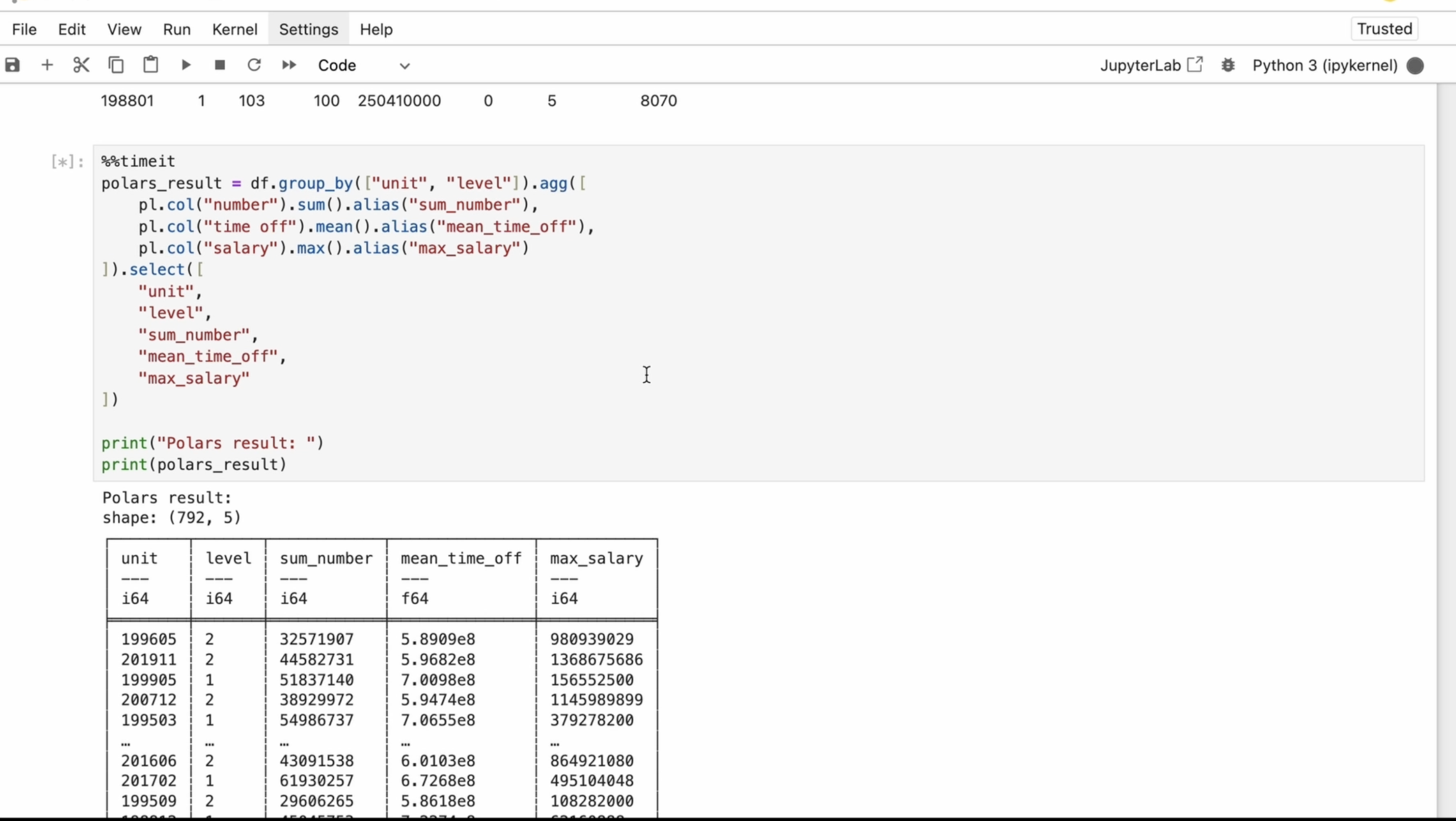
structured dataset, and I will proceed with grouping the dataset by the unit
and level columns. After grouping, I will perform
an aggregation operation on the number column by calculating the
sum of its values. First, I select the column named number from
the data frame. Then I use an aggregation
function that adds up all the values
in that column. Instead of keeping
the default name, I assign a more meaningful
name to the output column. For this, I use an alias. For time off, I'm
calculating the mean. For salary, I'm calculating
the max function. Finally, I will select the required columns from
the aggregated data frame. The select method and
polars is used to choose specific columns and apply
transformation to them. It creates a new data frame with only the selected columns, leaving the original
data frame unchanged. Sorry for typo. I use the print function to display
the result along with the heading in a
regular code editor. This is necessary
to see the output. However, in Gebr notebook, you don't need to print. You can simply type the
variable name, pole result, and it will automatically
display the result in an interactive
way. And here we are. Now, I'll use the time it command to run the
code several times. At the end, we will see how long it takes to
perform the operation. We see the code
running several times. And at the end, we find
that it took three dodge, 83 seconds per loop, or I can say per operation. Let's repeat the same
process with pandas. It takes more time
than with polars. We look at the same
data frame and need to rename the columns.
So let's do that. The command is almost
the same as with polars, except we define the columns first and then pass in
the new column names. Now we can proceed with the same grouping and
aggregation as we did above. We can see here that Pandas uses a dictionary inside
aggregation function to specify the column
names and operations. In polars, the aggregation
was applied to columns by selecting them first and then using functions like
sum mean and box. In polars, you cannot use
a dictionary directly inside the aggregation function in the same way as in Pandas. Polars requires you to specify each aggregation operation
explicitly for each column, and this is the difference. Pandas provides a shorter
syntax for aggregation. Both expressions will
give us the same result, but the syntax is slightly different between
Pandas and polars. I strongly recommend
trying it yourself. Pause the video and repeat
this code by yourself. This is what the final
table looks like. Now I will use time it again to run the
code several times. And it was run seven times. After running it, we see it
took 7.34 seconds per loop. We can clearly see
the difference. But we also need to
consider the cases when we perform these operations
along with reading the data. I will rewrite the
code just a bit. So we will read the CSV
file, rename the columns. Perform the group by
operation, aggregation, and then select
specific columns all in one chain using polars
method chaining syntax. This takes more time. And
now it took 11.8 seconds. Here, I re wrote the code for Pandas
to do the same thing. I combined all the steps into a single line just like we
did in the polars code above. Even without time it, I run it and my system runs
out of memory. Oh, yep, my system is dead. But we can manage this
even with Pandas. If we start reading the
CSV file in chunks, let me show you how we can
handle this situation. Reading the file in chunks
helps manage memory usage. First, I set the number
of rows to be read into memory at one time by
setting the chunk size. Then I initialize
an empty data frame that will store the final aggregation results
from each chunk. I read the CSV file in
chunks using the four loop, rename the columns, and perform the same grouping
and aggregation as before. At the end, I can coatenate the aggregated results from each chunk to the
final data frame. Also, I used Ignore index. True. This means that when performing operations
like concatenation, the original index values
will be ignored and the new default integer index will be assigned to the result. It helps avoid duplicate or
non sequential index values when modifying data frames. Here we can't break
the line like that. So I changed it for
better readability. It takes some time, but we
finally get the result. To avoid running out of memory, we can use MMIT a magic command from the memory profile package. It measures and pre ints the memory usage of the
current code execution. This helps monitor memory
usage for each chunk. In this version, MMIT is inside the for loop
before pre nt operation. It will execute in every
iteration of the loop. This is useful for analyzing and optimizing work
with large files, but it may slow
down code execution due to additional measurements. You can install it using PIP. Of course, you should use this command to enable it in a Jupiter
notebook environment. You use this command only once, not before each use of MMD. After that, you can use MMIT to check the
peak memory usage. Here we used this command for total memory consumption
of Pandas result. After all chunks we
have been processed. So if the goal is to check
the final memory usage, the second variant is better. If the goal is to track
memory consumption over time, the first variant is
more informative. However, we can avoid this issue entirely by using polars
instead of Pandas. Let's return to the
polars library. In the previous example, we
used read CSV from polars. This function reads the entire CSV file into
memory immediately, loading all data
into a data frame. So we can perform
operations on it directly. However, if the
CSV file is large, this approach can
consume a lot of memory, just like we saw with Pandas. But as I mentioned earlier, polars also has a lazy mode. If we check the type
of polars result now, we will see that it's a lazy frame instead
of regular data frame. With lazy evaluation
or lazy mode, we use SCNcSV
instead of readCSV. SCNcSV doesn't read the data
into memory immediately. Instead, it creates a
lazy frame which records transformations
and only executes them when explicitly triggered. This enables query optimization and more efficient execution. I copied the previous code and simply replaced readCSV with ScancSV if we check the
type of polars result now, we get a lazy frame instead
of regular data frame. Since lazy frames use
deferred execution, we can actually visualize the execution plan using
the show graph method. This method generates a graphical representation
of the query plan, helping us understand and debug the data
processing pipeline. It provides insights
into the steps and optimizations involved
in the query execution. To use Show graph, you need to have graph with installed
on your system. On MacOS, you can
install it using Brew install graph with
on Windows or Linux. You can check the
official documentation for the appropriate
installation command. Here you can choose the command for your
operation system. Looking at the query plan, we can see that only five out of eight columns
are being selected. This means that
polars only loads the required columns instead of reading the entire
dataset into memory. Next, I call HAD
on Polar'sRsult, and instead of getting
the actual data, we see naive query plan. This happens because lazy frames don't execute immediately. They just build the
execution plan. To actually execute the query, we need to call the collect. The collect method
triggers execution, processes all
operations, and returns the regular data frame
instead of a lazy frame. Since our dataset contains
more than 1 million rows, execution takes some time. At the end, we get the result. If we check the type
of our data frame now, we see that it's a
pulse data frame. Not a laser frame anymore. Now I copy the
previous code using Scan CSV and run
it with collect. Then measure execution
time with time. The code runs multiple times, and at the end, we
get the result. Let's compare this to
the previous execution. Using read CSV, the execution
took ten dot 7 seconds. There is no huge difference,
but look at this. If we enable streaming execution by setting streaming
equals true, in collect method, we process data incrementally instead of loading everything
into memory at once. Streaming execution is great for large datasets because it reduces memory usage by processing chunks instead
of the entire datasets, and it can potentially leverage
parallel processing where different chunks are processes on separate CPO course
simultaneously. Streaming execution generally
improves performance for large datasets by reducing memory usage and allowing
parallel processing. However, for small datasets, the difference may
be negligible. With polars, users
don't need to manually split their data into smaller chunks like
we did with Pandas. Polars handles it automatically. Now, we can see a significant
difference in performance.
10. Data Visualization in Polars. Advantages, Limitations, and a Comparative Analysis: When it comes to data
visualization and polars, it's often recommended
to convert your data frame to
a Pandas dataframe. As I mentioned earlier, we can use the two
Pandas method for it. Using Pandas for plotting
provides more flexibility. But you can also
use Matplotlip or Seaborne both widely
used libraries for data visualization. You can find video about these libraries in my
profile. You can check out. MD plot leap provides
more flexibility and allows fine tuned
control over plots. While Seaborn makes
it easier to create complex statistical plots with a simpler syntax and
better default styles. However, these aren't
the only options. You can also use HV plot, a high level plotting
library that works natively with
Polar's data frame. It offers a powerful
and flexible interface for creating interactive
visualizations. If you want to learn
more about HVPlot, you can check out
the documentation. Of course, you will need to install it first
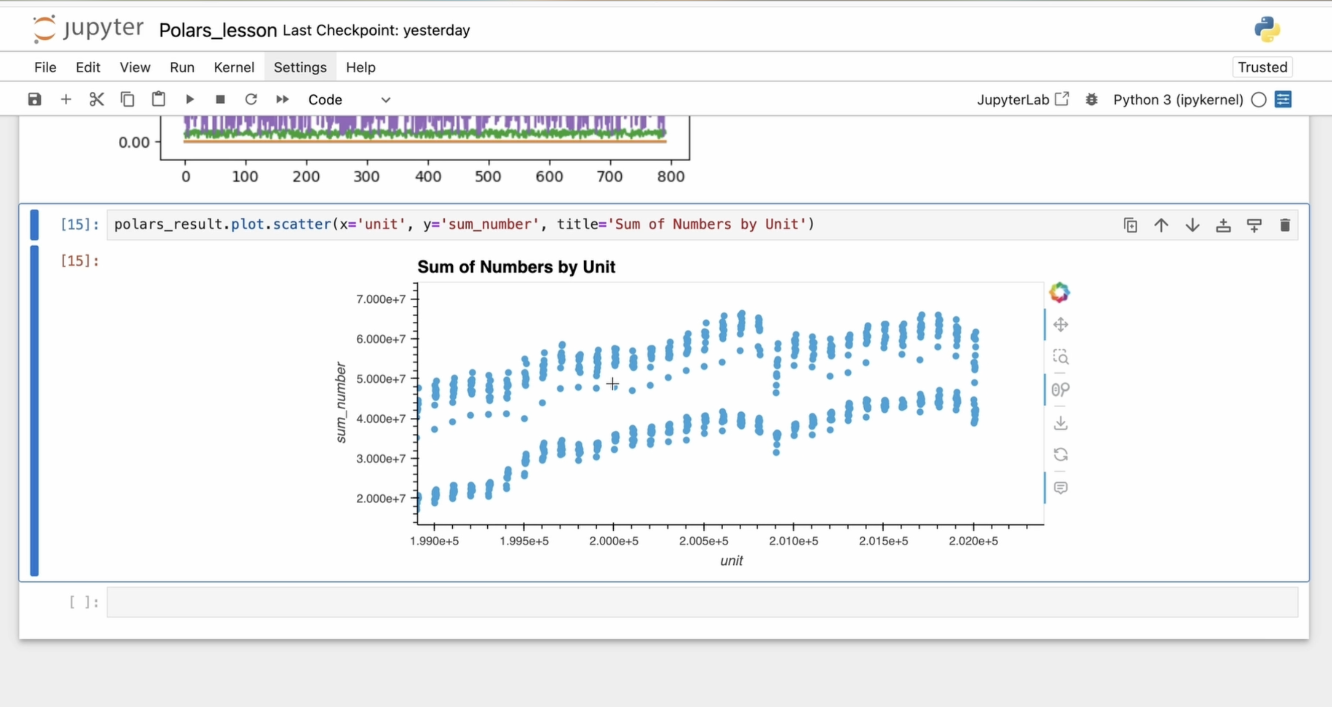
before using it. I polars, you can also use the built in plot
method to create basic visualization
without converting to pandas or using HV plot. The plot method understands
the structure of polars data frames and can generate plots using the
basic MD plot leap back end. You can specify
the type of plots, such as Scutter,
line or histogram. You also define column
names for the X axis and Y axis along with additional plot parameters
like the title. These types of plots are suitable for creating
simple visualization. However, keep in mind that the built in
plotting functionality in polars is limited compared to libraries like HV plot
or Mod plot Leap, which offers more
advanced features. For additional advantages, you may need to use
other libraries. So we have covered a lot today. While polars offers
many advantages, it also has some limitations and disadvantages. Let's
see what it is. First, polars is relatively new library
compared to Pandas, and it may not have as extensive community support or as many third party
extensions available. Pandas has a larger and more
established ecosystem with many third party
libraries and tools designed to work seamlessly
with Pandas data frames. Being a newer library, polars may not have
the same level of compatibility with existing data analysis libraries and tools. You should consider this before switching from the Pandas
library to polars. Another limitation
is that polars doesn't have the same level of indexing flexibility as Pandas. While it supports
row based indexing, it lacks the robust
multi level and hierarchical indexing
capabilities that Pandas offers. For example, in polars, you can only set a single
columns as the row index, whereas Pandas allows for more complex
indexing structures. If you have used multi level indexing in
your project before, this might be something to consider when
switching to polars. Additionally, visualization
capabilities in polars are currently
limited compared to Pandas. In Pandas, it's relatively straightforward to
visualize data directly from the data frame using
built in plotting methods or by seamlessly integrating with external
visualization libraries. So if visualization is crucial part of your
workflow and you don't need the
performance benefits of polars for your
specific use cases, Pandas might be more
convenient option for you. Switching from
Pandas to polars can potentially lead to
unexpected behavior or functionality gaps due
to the differences in the feature sets and capabilities
of the two libraries. As I mentioned earlier,
Pandas has been around for a longer time and has a more mature and
comprehensive set of features. While polars provides many essential data manipulation
and analysis functions, it may lack some of the
more advanced features or nice functionality
available in Pandas. So, guys, congratulations
to complete this course. You've done a good job.
Keep learning, keep coding. See you in the
next courses. Bye.
 Olha Al, Software engineer