Transcripts
1. Introduction: So over the last three
years being a student, I've tried all sorts
of money tracking magic spreadsheets and apps
did just don't work for me. Tracking money school for the first week and then my
brain just gives up on it. It's too much friction
and just boring. So I realized that in order
to make it easier for myself to see what I make
and spend in a month, I'm going to have to create
my own finance tracker. And to do that, I chose Google
Sheets as my tool. You see, over the years
of being a student, I got quite familiar with Excel and then later
Google Sheets. And so in this course, I'll show you the
basic skills and formulas that will allow you to create and customize your
own monthly finance tracker. First, I'll show you
how Google Sheets work, where to find them. Then you'll learn the
basic formulas and formatting options to help you create the finance tracker. And finally, I'll walk you
through step-by-step of how I created a monthly
expense tracker that works for my needs. This class is for complete
beginners to Finance and Google Sheets and doesn't require having any
prior knowledge. All you need is a computer and an Internet connection
to get started. And chances are if you're watching this,
you're already set. So if you're still open-minded
about becoming more fluent in Google Sheets and creating your own
finance tracker. Then I'll see you in
the first lesson.
2. Class Project: Great, welcome to this class. In this lesson,
I'll tell you about the class project and it's
going to be very simple. By the end of this class, I want you to create
your own Google Sheets, budget templates using
the key takeaways from this course and post
a screenshot of it in the project gallery
so others can take inspiration and see the
progress you've made. But the main thing that I want to emphasize here is that it's very important to try out new things as
you're learning them. You see our brains are not designed for keeping
information when we don't. To use, I encourage you to open Google Sheets and
go along with me pausing this class
along the way and trying the things I
show you yourself. That way, you're going to
improve your chances of actually remembering
something when you need to use
it in the future. And with all that said, I'll see you in the first
lesson where I'll show you how to get started
with Google Sheets.
3. Getting Started With Google Sheets: In this lesson,
I'll tell you about how to get started
with Google Sheets. So what are they? You can find Google Sheets if you go to sheets.google.com, it will open up a
new browser tab. The way sheets work is they're basically inside
of your browser. You have to login with your Google account
in order to see them. Google sheets basically live in your Google Drive account. If you want to access it, you can go to drive.google.com. And here you can see all
of my Google documents. You don't have to go through the drive to find the
Google Sheets every time. Just type in
sheets.google.com and you'll find them alternatively
in a new browser tab, you can click these
nine dots here, scroll down a little bit
and click on sheets to access your Google Sheets in order to create
a blank sheet, just click here and it'll
create a new sheet for you if you know anything
about Microsoft Excel, chances are those skills will transfer very well
to Google Sheets. And if there's a formula
that you use in Excel, it will probably work
in Google Sheets to. So first things first, the way you rename your sheet is go up here and then
type in the name. I'm going to name
this money tracker. Now whenever I go back
to sheets.google.com, you'll see that there it is. My money tracker. If I click on it, the
same sheet will open up. Now one cool thing
that you might want to do in order to access sheets quicker
from your computer is to either click
this star here, which will add Google
sheets in your bookmarks. So here you'll see them pop up every single time
you open your browser. Or alternatively, you can right-click on this
tab and click Pin and you'll notice that
this tab shrunk down every single time
you open your browser, this tab will open as well. So it's going to be permanently
pinned to your browser. And for a money tracker, this is very useful
and you'll be able to see all of your
finances at a glance. But if you don't want
to do that, no worries. Another cool thing about google Sheets is that you can
share it with others. So if you come up to
here and click Share, it'll allow you to copy
the link of this sheet. You can also click here, say anyone with the link. And then instead of
viewer, choose editor. And now whenever you share
this link with someone else, they're going to be able to make changes to your Google Sheet. If you choose viewer. They're only going to be able
to see what's in the sheet, but not actually
edit its contents. Now, if you're completely
unfamiliar with sheets and don't know what
all of this stuff is, all these formatting
options and stuff. The best tip that
I can give is to use this help menu over here. So if you want to change
something or insert something, maybe there's a formula
that you want to find. You can just put it in here and Google sheets will
automatically find it for you. E.g. if I want to add
some cells together, I'm just going to say sum and is going to give me
a lot of options here, inserted the sum function, so my function and many others. So basically if you're stuck and don't know how to do something, just use the help function
or if you're on Mac, click Option and backslash to immediately jumped
to the help function and start typing something. If you've used Google
Sheets or Excel before, you'll know that formulas
are a very big part of it. And so in the next lesson, I'll run you through
the basic formulas that you'll need for
tracking your finances. I'll see you there.
4. Mastering Formulas: In this lesson,
I'll tell you about how formulas work
in Google sheets. Formulas are basically
the backbone of how Google sheets
or Excel works. So learning them will
help you improve your workflow by ten times
at least what our formulas. When you step on
a cell in Excel, you can either type in it
directly or you can put equals. And this means that
you're going to type some sort of
a formula, e.g. you can type equals
three plus seven, and once you hit Enter, it's going to spit out a ten. Now, if you go
back to that cell, you'll notice that up here
in the formula field, it actually shows the
formula in the cell. It shows the outcome
of that formula. What you can also do is drag formulas down to apply
them to other cells. So if I click this
little rectangle here and drag this formula down, it's going to put ten
in every single row. And you'll see the formula
is equals three plus seven. Now if I change this one, the second one into
three times ten, it's going to be 30 and then highlight both of
them and drag down. It should repeat the pattern. So Google Sheets
recognizes that it was ten before and after, and I went to duplicate that,
duplicates the pattern. Of course, some complicated
patterns will not work, but if they're simple enough, google Sheets will
understand it. We've learned how to
add basic numbers, but what happens if you have, let's say a lot of
numbers here and then you want to
add all of them up, but show the results, e.g. in C1 in this cell. For addition, there's a
formula called a sum. So you're going to
type equals again to start the formula,
some open bracket. And then what's really useful is Google Sheets will always
tell you what to put in next. It needs a value, so let's say one. Then you're going to put a comma and it needs
a second value. So I'm going to see two. If I click Enter now
it puts out a three, which means that it
added up one to two, which equals to three. Now what you can also do with the sum function is
type equals sum, open brackets, and select all the numbers that you
want to add up together. So if I select all of
them, click Enter, it's going to spit out 78, which is the sum of
all these numbers. Now the next cool formula
is called unique. It basically lets you find one-of-a-kind values
from your data. This will be useful later because we're going
to want to add up individual categories in
our finance tracker, e.g. if I have all these words here, some of them are repeating
and some of them are not. And I come here, equals unique, and then
select all of these here. It'll spit out only the
ones that are unique. It's not going to
repeat dog twice. You can see how this
might be useful later, two separate specific categories within your finance tracker. And the next formula, which is probably the
hardest one is called sum. If it basically adds up cells based on if it fits a
certain criteria, e.g. if I have all of these
animal names again, and then I have a
number beside each one. Let's say the number is
ten for all of them, I can type equals sum F, then it tells me
to select a range. So orange would be animal names. Then I'm going to put a comma. Now it's asking me for
a criteria, basically, which one of these animals do
I want to add up together? I'm just going to click on dog, is going to look at
all of these animals, then pick out dogs and add up all of the
numbers for the dogs. Let's see, there
are 123456 dogs, so the number should
be 60 at the end. Then I'm going to put comma, tell Google Sheets
what I wanted to add. So it's basically all of these numbers and
if I click Enter, it should spit out a 60. So again, what happened
here is first of all, we selected all of
our categories, so all of the animals. Then we told Google Sheets, which one do we want
to add up together? And then I finally showed
the numbers which it should add up to if
the category fits dog, I can also choose a
different criteria, so e.g. cat, and it's going to sum up all the numbers besides Cat. So let's see how
many cats there are. 123.4. So the number is
40, so somewhat unique. And some IF functions are
the ones that are going to be very useful for
making the finance tracker. In the next lesson, I'll show you how to
make your Excel sheet beautiful by using
conditional formatting. See you there.
5. Understanding Conditional Formatting: In this lesson, you're going to learn about conditional
formatting, which basically
lets you change how a cell looks based on
what's inside of it. E.g. you can specify that if a value in a cell
is less than zero, it's going to be colored red. Or if the value is
greater than zero, it's going to be colored
green. Here's how to do that. Let's type in a few
values here, e.g. ten minus three Enter and
let's put something like dog, say something random,
something random. Now I'm going to
select all of them, go to Format and then
conditional formatting. It's going to open this panel
over here on the right. By default, if the
cell is not empty, it's going to format it
by adding a green color. And we can change
that, Let's say e.g. that I want to color only
the cells that are greater than zero green and leave
the others just blank. I'm going to come here, Format Cells F and
search for greater than, their desk, greater than. And then I'm going
to input zero. And you can immediately see the changes happening
in the sheets, so only the ten has the color. Now. Now what if I want to color
the cell that says dog, e.g. orange, I can come all the way down and click add another rule. Then in the format cells, if I'm going to choose texts, contains, and type in dog, and then I'm going to change
the formatting to orange. You can see that the cell
that had dog is now orange. So now if I change
minus two into e.g. three, it's going to become green since it's
greater than zero. And if I change
something to dog, It's going to become orange
because it says dog, I can also drag
these cells down and it's going to carry its
conditional formatting with them. So e.g. if I type
minus two here, it's going to become
just a blank. Now you can go back into
Conditional Formatting and add more rules or delete
rules if you want to. So these are the basics of
conditional formatting. And in the next lesson we're going to apply all the formulas, tricks we've learned
so far to build our own finance
Tracker template. See you there.
6. Practice: Creating A Finance Tracker Template: In this lesson, we're
going to be creating a simple finance Tracker
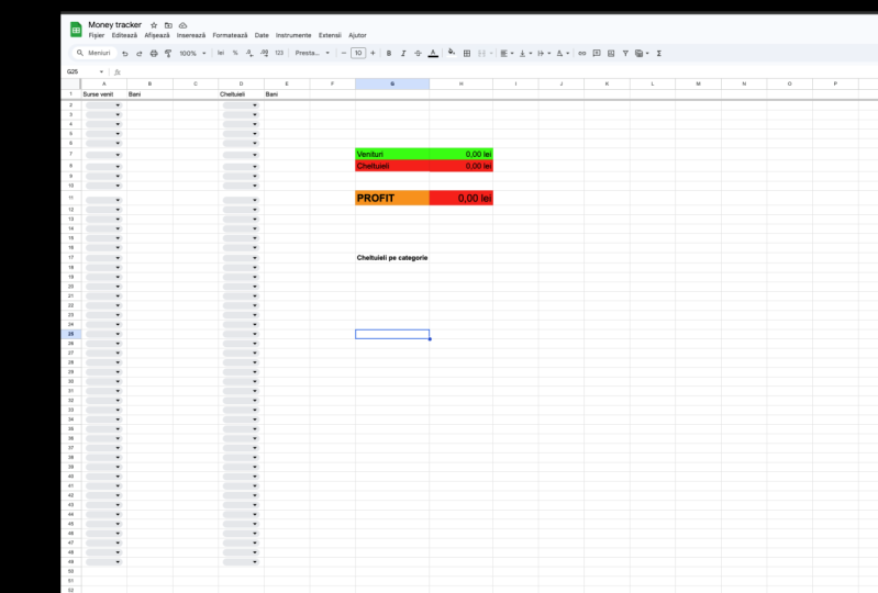
template in Google sheets. First things first, I'm
going to type sheets dot new to create a
brand new Google Sheet. I'm going to name
it money tracker. Then in the A1 cell, I'm going to put a category. Next, I'm going to put income, category and expense
in the A2 cell. I'm going to right-click, scroll down and
choose drop-down. This will allow me to create
categories for my income. So over here on the right, I can specify the categories. So let's say job than, let's say the second income
category is side hustle. You can also choose different colors for each
of these categories. It's just going to be
easier to differentiate between them when you
pick them afterwards. By the way, you
can always go back in here and change
everything later. Click Done, and
then come back to the category and drag it down. Let's just cover 100 cells
in the expense category. Again, right-click,
go to drop-down and specify your
expense categories. Here you'll probably have
a lot more of these. E.g. utility's going out, clothing, food,
subscriptions, and so on. Click Done. And again, come back
here and drag them down so it matches the length
of the income categories. Now, select B, which is going to highlight the
whole income column. And then in the format here, click Format as currency, do the same for the
expense column. Now, whenever you input
a number here, e.g. 500, it's going to
format it as dollars. Then I can come here
in the category and categorize these
$500 as job income. I can do the exact same
for my expenses. So e.g. $30, I can come here and
choose subscriptions. Now if you what
the category says, you can simply expand the cell. Next, I'm going to highlight the first row by clicking
on this one here, come up to view, freeze and then one row, this is going to freeze the first row so that
when I scroll down, it's going to stay at the top. I'm just going to add a
few more expenses here. So it's going to be easier to visualize what we're gonna
do next, okay, next, over to the side here, type income than expenses
and then savings. This is going to be
the summary of all of your categories to the right
of income type equals. This is going to be a formula, some open bracket, and then
select all of your income. And this is going to sum up every single cell in
the Income column. If I add another
source of income, e.g. $50, it's going to update
and say 550 in the summary. Now in the expenses column type equals sum and do
the exact same. But for the expense column, once you click Enter, it's going to sum up
all of your expenses. The savings will show us how much we've saved this month type equals select income
minus expenses and enter. Now I want to make my savings
look nice if they're above zero and look not so nice
if they are below zero. So I'm going to click
the savings cell. You do format and
Conditional Formatting. Then in the format cells, if I'm going to select
greater than and type zero, which will color
my savings green. If they're greater than zero, then I'm going to scroll down all the way and click
add another rule. Now I'm going to choose
less than or equal to zero and change the
formatting to read and click. Done. So now, if I
add more expenses and my expenses actually
are higher than my income, the receiving cell,
it will turn red. Now next up, I want
to see how much I spent for each
category in total. So e.g. how much I
spent on food in total, since I'm not going to go
here and calculate each one. And for that, we're
going to use the unique and some IF functions
that we learned earlier. I'm going to come down here
and say expenses by category. I can also highlight all of these cells and make them bold by pressing Command and V or Control V if
you're on Windows, now I'm going to move one
cell down and type equals unique open bracket and select all of the
expense categories, but make sure not to
include the word category. And there we go,
it wrote out all of the categories
that are unique. Next, I want to add up the expenses for each
of these categories. And for that, I'll use the
sum f function equals sum if open bracket and it needs a range and the
range is our categories. So I'm just going to select the C column to select
all of it now comma. And it asks me for a criteria
which is going to be this expense category than comma and some range
are the expenses, the D column to select
all of it and enter. Now, Google Sheets automatically
asked me if I want to auto-fill the other
categories I'm going to choose, know, then come up to
the cell where I wrote the formula and actually just
drag it down all the way. The reason I just did
that is because if I add another category year that
has not yet been used, e.g. utilities, the unique function is going to add one
up automatically. And then if I type in an
expense for utilities, it's going to count it up
automatically as well. Now you'll notice that
there are a bunch of zeros here that I
don't want to see. And for that, again, we can use the
conditional formatting I can come up to here, select the first cell
and then click Command, Shift Down Arrow to
select everything up until the very bottom cell
that has something in it. You can use control shift
down arrow on Windows. Now, I'm going to come
up to Format and say conditional formatting
here in the format cells. If field, I'm going to choose
equal to type in zero. Now you'll see that
only the cells that have zeros are affected. And then I'm just going
to pick white here and white text color to
just make them invisible. I'm going to click done, and now the zeros
are not visible. So whenever I add a
new expense, e.g. let's say 1,000 in the
utilities category. It's now automatically
going to show me the sum of all my utilities in
the expense column, there are two total
categories for utilities and the some
of them are 1,100. And that's what I see here. Also, I can select the
hundred click Command, Shift down arrow again to select every cell that
has something in it, and choose this dollar sign
to format it as dollars. And this is my income and
expense tracker for the month. But what happens when this month ends and another one
begins for that, I want to create a template
so I don't have to do all this work of recreating
it again for the next month, I'm going to highlight
my expenses and income and click Delete
to remove all of them. Then at the bottom, I'm going to double-click on this sheet and name it template. Now I will never touch
the template sheet again. Whenever a new month starts, I'm going to right-click
and choose duplicate. I'm going to rename the copy of the template with the
current month and year, and then I can simply
move it to the left. So for the whole
month of February, I'm just going to use
this February sheet. And whenever another
month comes around, I'm going to right-click
on the template, duplicate it again, rename it, drag it to the beginning. And here I'll have a fresh new monthly tracker for the next month.
And that's it. You can modify this
template however you like and use it to track
your own finances. Because what gets
measured gets improved.
7. Sharing Google Sheets With Others: In this lesson, I'll
show you how to share your finance template with your friends or anyone
else to do that, go over here to share copy link, open a new tab in
your browser and paste the link with
Control or Command V. Then you're going
to want to delete everything up until this
last slash over here. So everything from edit onwards, you should delete and then
just put Copy instead. Now, highlight all
of this link with Command or Control a
and copy it again. Then you can send
this link to someone. And once they click on it, they will be able
to make a copy of your finance Tracker
template for themselves. That way you're not
going to be working on the same exact document and changing up each
other's finances, but each have a separate
customizable finance template.
8. Conclusion: So you've reached the
end of this class. Big congratulations for me, and I hope there's at least
one thing that you'll take away from it and
use in your own life. Of course, the best
thing when trying to learn new things is
to put them to use. Because if you know a
formula exists in your mind, then there's a very
high chance you'll forget it if you don't
use it over time. That's why I encourage
you to share a screenshot of the
finance template that you've made by
applying the things you learn in this class in
the project gallery. And just one more thing, if this was helpful, Could you do me a
favor and helped me improve by leaving a
review for this class. Just out of curiosity, I want to know what
you thought about it. I hope that you enjoyed it and gain some knowledge from it. Thank you once again, good luck and I'll see you in
the future course.
 Thaomaoh, Learn Creatorpreneur Skills