Parametric Design with Grasshopper Full Beginner to Advanced

1. Course Introduction: Hello and welcome everyone to the parametric design with Grasshopper course. My name is Jeff. I am a Senior Architect, parametric designer and BIM Manager with many years of experience using and teaching grasshopper. My first experience with grasshopper was during my master's degree in the USA, where I and my colleagues do not only use Grasshopper to design, but also the fabricated and build an avian observatory from scratch. The whole process from initial design, fabrication was made possible with Grasshopper, especially that the building elements were all unique and parametrically driven. I have been since using grasshopper on a daily basis, solving complex geometric problems in a streamed line strategy and providing early design solutions while combining it with BIM using Rhino inside Revit, as well as other parametric tools. My teaching passion found its way first at the FabLab Berlin, as well as other design companies, institutions and universities in Germany and Europe. Participants from all over the world with various design backgrounds joined my courses and benefited tremendously from them and are able to implement their knowledge in their studies and professional career. The course is divided into eight units, starting from the beginner than intermediate and ending up with advanced levels. You will learn not only what grasshopper can do, but also how to efficiently use it and what are the best methods that allow you to solve complex design issues quickly and efficiently. The total length of the course is around 16 h. I highly recommend practicing daily grasshopper. Since the best way of learning it is by doing, making mistakes along the way, understanding how it works and learning from that to reach new levels. You will be able to download all the course files that include detailed explanations as well as all the components. Practical examples, optional but recommended assignments and exercises. Whether you are an architect, engineer from all fields, a designer from all fields, including but not limited to product design, jewelry design, fashion design, graphic design, or a student of these fields, Grasshopper would be a great addition to your toolbox. And we'll push your design abilities to a whole new level. Alright, if you want to learn how to use this amazing parametric platform, get on board and let's get started. 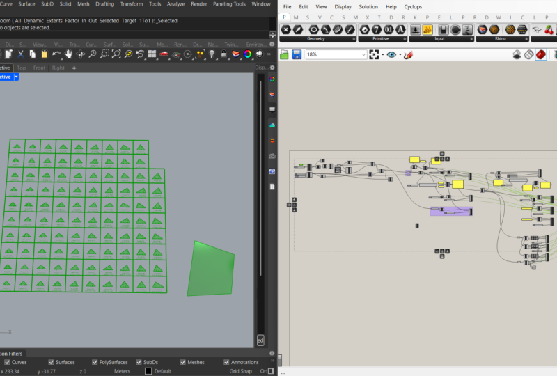2. Interface: Alright, so the course is organized in this way. So we have several unit classes. And for each unit class we have a Rhino file and a grasshopper file. Inside of each grasshopper file, there is some content and definitions and components that match the Rhino file. So now let's launch the first unit one class Rhino file. Alright, so this is the mono file and you can see here we have few layers with few geometry is already made within. Now, grasshopper is a plugin to rhinoceros. It's kind of like a small separate software that you have to launch. There are two ways. Either we can here in the command line type, grasshopper, and then enter. This was actually the old way with Rhino versions prior to six or 5.4 and the ones before, where we had to actually install grasshopper after installing rhinoceros and then launch it from there. However, starting from rhino six, we already have now this icon where grasshopper actually is already coming with Rhino. So I can also click on this icon to launch grasshopper. Here. We have now with this new window that you can see that opens up. And also it has its own like, like toolbar here and here, like some more tabs and sub-tabs or sub menu tabs. And when you first launch a grasshopper window, you will have here at the beginning, like these previously opened grasshopper files. For now, let's instead of clicking on one of these and not get confused if it was the correct one or not. I'm going to directly now drag and drop this one. So the unit one class grasshopper file.js, drag-and-drop will minimize this one. So now you can see this is the grasshopper file. I'm going to maximize this window. First of all, I want to first explain about the grasshopper file organization as well. Inside of each file, we have topics that I'm explaining about. So e.g. now starting with the first unit, we have the interface referencing points, constructing points, etc. For each topic, wherever I am now explaining to you orally, there is a summary, brief points about each topic. So you can actually go back to these if let's say you don't have any more access to the recording or maybe for some reason offline or two or anything, any reason then. But however you have the files, you can still go back to the file. You can go to these panels with text explanations, brief summary about what's coming on, the what's happening. Here. Let's say there's more detail explanation about vectors, e.g. so you can actually will go back to these panels and then get more in detail about the summarized points and topics and ideas. Alright, so let's start now with the interface. So as I said before, the definition window, this one called definition window, the grasshopper window is inside of rhino. I mean, of course I can now nudge this one to this side and this one to this side. So I can have, let say, two windows next to each other, e.g. this is something that's personal preference that you can make, but you have to know that it's a different window to separate window that opens up in which you work on this canvas inside of this grasshopper field. And then you will see the preview of your geometries of your resultant happening inside of this viewport of rhino here. So would it be in perspective or top or any view you will see the preview of what's going on here. Then at the end, when you are satisfied with the results and you are done, then we can do something called bake, which will actually bring the geometries or the definition, the product that result from Grasshopper into Rhino. Now we're going to talk about this later on, but for now, just understand that this is a separate window of Grasshopper. We work here. We see here the preview. We see the result of our work progressing. Once it's done and satisfied, then we can bring it back here. We are not actually live updating the baked or the geometries, but just updating the preview and the process here, we can actually open multiple definitions and switching between them. So now I have opened the unit one class. Now I can also open another unit or many more units, files or minimal grasshopper files. Inside of this same Rhino file, I can simply go to this folder. Now, drag and drop the unit to class here. E.g. is something that is possible. Alright? And when I do that, then if I want to switch and go back to the unit one class, I can click Go bacteria and then click on this one class. Now I can switch between the grasshopper files that are open inside of this same Rhino file. Or with this random file. Now, if I want, let's say to close one of these, because I don't want to use this one. I can go to here. And I can click on this. X becomes red. When I hover over this, I click and I close it. Alright, so that's how I can open multiple definitions and also close them. Now, what about the top menu? So here we have this top menu here, wherever they like the standard buttons, we're going to actually to go deeper and explain some of these commands and buttons when we reach them throughout the course. But for now, just understand that we have these ones here. Actually this is, this bank is a plugin that already installed inside of grasshopper. So it's actually a plug-in to grasshopper, which is plugged into our answers. We're going to see also later on and talk more about plug-ins that are made specifically for Grasshopper. We have the tabs, these ones. So we have perimeters, maths, sets, vector, curves, surfaces, mesh, intersect, Transform, and display. Until here, the display. If I now actually maximize this one, it will display this. These are all the native grasshopper tabs. Now, everything else that comes after displays, pufferfish, weaver, bird banding towards etc. All of these ones are installed plugins to Grasshopper. We have the visibility options on this top right side here. The vector meters. So you can actually hover over these and check out what these do. So if I hover this one and I activated, only draw any, don't, so don't draw any of geometry. So if I'm working now and even if I have some junctions that have their preview on or there are turned on and should be visible here. If I turn, activate this one, then it will actually not show me anything. This is to draw wire-frame preview geometry. And this is to draw shaded preview geometry. I usually keep this on. Here we have this one which mean so draw a preview boundary on the Canvas, exclude objects. Then it says your press Escape to remove any distinct boundary. What this does is that e.g. if, let's say I have this privilege geometry on, this turned off. So I'm going to talk about this. So now I have this point and have these points for instance, like these have the preview on. Also talk about the previous settings shortly. If I use this one and I draw, if I click and I draw something like that, it will only draw what is inside of this virtual area. Let's say. If I click on escape, will then activate that one and then show me again what should be scene. If I click on this again and I do this. So there's nothing inside of this area now. I'm seeing nothing. Only previews to me or shows me what's inside of this area. And of course it should have the preview on setting. If I click on Escape, now it goes back to what it should be showing me normally. Now what about this one? This says only draw preview geometry for selected objects. This means that if I click on this one now I have nothing selected. It will show me nothing. If I click on this component, it only has one point. I'm seeing now, one point, multiple points. These are here three points, e.g. right. So it's only showing me what is being selected. If I deselect this one, then it's showing me only what, which components have their preview on setting. I'm repeating this preview or several times, we're going to reach this one soon. Actually in Grasshopper, there are many ways of seeing things like preview of the components or the way to show things in and out of between grasshopper and Rhino. So bear with me shortly with this. I'm going to show you what these do. And you will see actually with practice and experience that you will find this really helpful and practical. You will be switching between them on and off while working, depending on what you want to do and what you want to see actually why working. Let's go back to here. So these are an option as well. So the remaining 21, so this is the document preview settings. If I click on this, in general, by default, we have the normal color of components that is in breadth, of course, with a slight transparency and this one in green. Now you can change these ones. This means that when I have a point and it's not being selected, but it's on, it will be in red. When IT sector, then it's going to be in green. So if I go back to this one, normal selected, I can change this color, e.g. I'm not, I'm not going to change it and keep it to default settings, but you can go back to here and change per your personal preference. This one, the last component, the last item here for previewing information and data and geometries is this one. So it's repeat view mesh quality. You can go back, you can go here and then you can either disabled dimensioning or say, low-quality, high-quality document, etc. And then customize the qualities. And this becomes handy. Let's say if you have like a really large File and complex geometries and it might be kind of flex slowing down your file, then you can use low quality. Or actually you want to show high-quality geometries, then you can turn on this one. I'm going to now keep it to low-quality. Now, on the top left, open here we have this. You can open the new grass or profile here to save the file. This is the zoom factor here. So it's how much I'm zooming n. This is the view entire document. This will take, if I click on this and goes and I click on this one, it will focus on the upper left. If I click, I'm going to undo this one. I think I moved it. I'm going to click on this one. It will zoom to extend, let's say, to all of the components inside of this file. Let's go to here, we have the main views, these ones. So e.g. let's say that I want to save this position. How I'm seeing now the Grasshopper definition components. I can click on here and I can now say like maybe this is called referencing points. Let's say I will, my name is referencing points. And I will say, okay, now if I now Ben and move away and zoom in and out, etc, like this, I can click on this drop-down arrow and I click on this one. It will take me again to the same position in the same Zoom where I saved it. So there's something interesting that you can actually save kind of positions inside of grasshopper. And this last one, you can actually sketch on this Canvas. So you can see, I can click here and I can sketch whatever you want to sketch. You can change the thickness. You can change the color of the line. Okay? Right-click can even simplify it to make it curvy, less polyline style, but more spline slide, e.g. this becomes handy. Let's say if you want to kind of sketch over some ideas like e.g. I've used this. What does sketch e.g. this idea about the vectors in 3D, the X, Y, Z vectors. So I just sketch these ones with using this tool. Basically, it becomes handy to sketch over some ideas that you want to while working to quickly kind of save your ideas. And in this way. Now, at the bottom left here, you will see, while working, you will see the recently used commands here. Now we have nothing because we're still just launched grasshopper. With time. Now while working, you're going to see now this one with the latest commands used. This at this side at the bottom right, we have this navigation campus. Now, this campus is useful, Let's say if you have a really big file and then suddenly like for some reason like you are zoomed in somewhere where you don't see anything and you kind of zoom in and out and you are going to floss then you know where you are. Then you can look at this campus. And this will point out at all of the components inside of the grasshopper file. So it can move this way. Now, I am not lost anymore. So you see these are going to point out at all of the components. You can actually move it around if you want to keep it there. I can actually turn it off by going into display and going to I think get this Widgets and encompass. Now it's off. I'll keep it off. Alright. Now, what if you have a fork, a moderator that are using on your computer or laptop screen, and then this might cause some issues. Might, I'm saying, I'm not certainly do that in terms of the font sizes. In case you find some font issues where text fonts inside of dependencies wrong, too large or too small. Then please make sure to download the pancake plug-in and reset all font sizes. Visit the thread where it was discussed about this, the download link to the plugin. And basically, let's say sometimes it might happen if you have, let's say, different monitor definitions or sizes that e.g. like this would become something like this. I'm gonna change this one just for the sake of the example. Do something like that, e.g. like this. So it becomes like really out of scale, right? So I can go to this one. Once installed pancake, then you will get, you will see this new toolbar. You can go to adjust font sizes and you can click on reset all. Then it will reset all of the fonts sizes. You can actually increase the sizes of all of them, or decrease the sizes. Or reset, reset all, reset all of the font size of the panels to eight. This is the standard size of settings custom for this to eight points, that's the font. Standard size. This is for you in the beginning, just like putting this in the very beginning. In case you face any issues, then please make sure to download this plugin and then do this. It is just like save a lot of time on adjusting the font sizes. Alright, now, let's move on to referencing points. 3. Referencing Points: Alright, now let's look how we can link geometry from Rhino to grasshopper. This process is called referencing, and in this case now we're referencing points from Rhino to grasshopper. By the way, all of the explanation that now you're hearing is here summarized in text form inside of this petal. I'm going now to turn on the one-point player. And I want now to reference this point from Rhino to grasshopper. I need now to find the component that can actually reference, can read this point from Rhino. And this component is called point basically. And it's under perimeters. Geometry. Point. By the way, all of these components under Geometry look like this. They are black hexagons with the symbol of the element and white. So for the point we have a hexagon with a white X for the vector of black hexagon with the white arrow, et cetera. These are used for either referencing or a shortcuts inside of grasshopper. I'm going to click on point and click. And now I get this new component point. Inside of a grasshopper. What if, I don't know where this component is actually here in under the tablets, maybe it's like other set somewhere e.g. n. Is like there and I don't know where it is Exactly and I'm searching and I can't find it, then you can actually search for it. You can double-click. And now you get this temporary search field, enter a search keyword. And then now you can type in the title of the components. So I can now type point B 0. You see now while typing the letters grasshoppers trying to guess what I want. So when you are typing, then it's trying to narrow down the components options that are in there that can match what I want. So n t, alright, and then I will have all of these options, all of these components that include within their name. And this case I want the point, I can click on this one and I get this component. This is really similar to the Rhino command field, but this is now here fixed. Second I type T 0 N T, right? And again, get all of these options that are available inside of rhino. Here I can double-click again, do the same, d and t, and I get the same, but this is temporary, so it's not fixed inside of grasshopper. I'm going to delete this one. I have already made this one. So this component, as you can see here, is now not referenced yet. We just brought it in from this here or while searching for it, but it's now an orange. And we get this information when you hover over this, it says, zero point contains a collection of three-dimensional points, and under that it says empty point perimeter. This pop-up message as well as the same. So floating perimeter point failed to collect data. You can also click on this. It has the same. So this is now the method, the message that we're getting. And this is now an empty component that needs to be fed in width information with a point. In this case, I can select this point. I can right-click on this component. I can click on Set one point. Now, once I do that, now this becomes white and the pop-up message now disappears. Then now this point is now referenced inside of this component. You can see now if I turn off the layer from Rhino and I click on this now I can see the preview of this point inside of the viewport of rhino. Alright, so I'm going to clear this value. I want now to de-reference. I want to detach this point from this component because I want to keep this as unreferenced, not for you as to understand what's going on. So I will right-click and click on Clear values. Alright, This goes back to the orange color with this pop-up message. This is the same as previous one, so it has now the points referenced inside of it, this one. What if I want to reference multiple points? In this case, I will now turn on the layer multiple points. And here we have three points. If I bring component point and I right-click on this while these being selected, I right-click and I click on set multiple points. Now I get all of these three points referenced under this component. This is the same as this one I already made here. So I will delete this one. You can see that both components, although they are referencing different points, they include different points, but they look exactly the same. Like even when I referenced multiple points here and it got these three points. It doesn't now get an S. Doesn't say points, still point, it doesn't change its name. However, there are totally different, although they look exactly the same. So be careful about that. That even if you have, let's say, one component, sometimes in Grasshopper, it does not mean that it holds only one element, but it might include hundreds and even thousands of elements. So just be aware of that. Now, you see that what's happened now is that we got a new component like this. It wasn't orange. When we referenced it with the information with data with geometry from Rhino, it became what? It changed colors. This color changing is really helpful. And grasshopper, it helps us understand what's going on. I'm going to delete this one. This is called color-coding. We have different colors that Grasshopper helps us use us to help us understand what's going on. The first one is the orange. So orange means empty. The red means it's an error. So in this case now I'm using here linking this one with the Boolean toggle false. This, we're going to look at this later on with the consent of the course. But for now I'm just using this one as an example. Because now this component is expecting to have a point, link to it are referencing a point, but it's getting a false message basically. That's why this is becoming red. So it's saying, Hey, there's a big error. I'm not even empty, but I'm giving, I'm being given a really false information doesn't work. We have the white that we saw previously, so it looks like white enabled and showing gray enabled. And no preview. So great with black text. What this means is now previa no preview. Let's look at this now for a moment. In this example, I actually was having these showing you these were not selected. Then we saw nothing, we see nothing. Why? Because this is activated, this only drop review geometry for selected objects is on. If I deselect this one, if I deactivated. Then now we can see the preview of the points in red. On when I select them, then I see the selected point in green. So this component now in green, if I de-select it in red. This is now showing me that only the components that have the preview on. So right-click, make sure that preview is on. If this preview if is off, if I do this one right-click and preview off and this one as well, because that's the multiple points of now I don't see them. If I select them, even if I select this one, I don't see the preview inside of the viewport of rhino. While this one I can see it when it's not selected in red and one selected in green. Now, if I turn on this one activity, this one, this will show me whatever is being selected, either TASB review on or off. So now I have nothing selected here. I have nothing selected. I see nothing. If I select this one, I see it. If I select this one, I see it. I see the points, even if this has the preview off. Alright, so when this is activated, it will show me whatever it's only being selected V it preview on, preview off. If this is not activated, it will always show me what it's Preview on and read when it's unselected and when selected in green. Alright, so now if I turn this back again to preview on, I can now see it. And now the preview shows me the component in twice. So this is how it's helping me, grasshopper, understand what's going on. So the components that have the white color have enabled means that are working and their PV is on. When it's in gray with black text, it's enabled and no preview, preview off with when it's kind of slightly faded and then detects this favorite as well. This means they are disabled. So this means that this components actually not running at all. Sometimes you might use this one for, let's say, like components are really heavy, that you're calculating, computing big steps. And they might, maybe slow down your Grasshopper definition, your workflow. Then you might want to disable them temporarily for while working. So you can right-click, you can click on enabled to enable them. Again here to disable that. So this is now disabled. That's why you can't even see them. So these are five ways of how you can see the components, their colors with either orange, that's empty, red, error, white, it's enabled and preview on. Gray. It's enabled the preview off and faded. Then it's turned off. It's not any of this, this eight. Alright. Now, even in third layer of how grasshopper shows you components is actually by either showing you their name or their icon. And in this case here, now you can see most of the components inside of the definition have their names. They are shown. And this is because I have here from the display not activated draw icons. Here. I also have draw a full names. If let's say I don't give, don't activate, draw a full names. It will only show you XYZ. But for the sake of explanation, also for your sake of your For your learning and you're activating draw full name so that you can, or you see the full names of the inputs are x coordinate, y coordinate, etc. And this helps you understand and learn better and faster at the beginning. But let's go back to this one. So I said that here I don't have this dry icons on. And so it's showing me the names. This is like the system settings of the file. But if I want, even though I have this setting being done like this, not activated, I can still make them few components show their icons. I can click right-click and I can click here. So always draw icon. I can click on this one. Application Settings. So this is the application, something that is now being used to only draw the name or always draw name. So use application setting is one option. Or always draw name if, let's say even your application setting is always draw icons than this one. It would show you only the name or always try icon. It will either it's a personal preference actually, depends on you, what you want, what you would like to, how you would like to work with the grasshopper. Sometimes people like to work with the grasshopper with their names of the components, sometimes with the icons. It depends. I personally prefer to have the names because I usually work with them as like I remember them, understand them by their names, by their function, and not by their icons. But you can also use the icons if you want. You can go to display and then click on this one to change all of the components displayed two icons. We saw this, the Boolean toggle false to make this error only in this case they're showing you the example. Now grouping. So you can actually group multiple components inside of grasshopper together. This is not geometric grouping. You are not, let's say grouping curves together or points together or like it's unlike grouping geometries, which is just now here, drooping components together. And this is simply done by selecting the components and click on Control G. That's one way. First way, I will now delete the school by selecting it and deleting or select the group, Right-click, click on Group. I will undo this one or select the group. Click on the wheel, and click on group. This third way and forth way, you can select it. They've components. You can go to Edit, Group and you can group them. So there are many ways of grouping components. Not only you can route components, but you can also when you group them, now you can see we have the group, but it doesn't have a title. You can give it a title. So we can right-click on the group. And you can say e.g. right. This really comes in handy when, let's say you have different components that are doing something and another group of components doing something else. So you can group them to say, Hey, this group of components is maybe building the facade of the building, or it's maybe making the handle of the door or something. So be it an engineering product design are that should in any field, you can group components just to remember what's going on, what they are doing. You can change the way of how the group looks like by right-clicking on the group and chasing using these options. Box outline. This is like the standard one. Or you can use Blob outline. Or you can also use rectangular outline here. So different ways of showing the groups. And you can also use subgroups. You can, let's say, group two components together than group these ones, this group was another component to have a subgroup with a bigger group. You can see here we have different colors of the groups. This is really easy. You can change it really easily by right-clicking. Go to color, and then change the color. So maybe I want this to be red, full rate and then no transparency. E.g. this could be an option, right? You can go to color, change something to say something else. Saturation. You can just play with these parameters there. Now, if I want, let's say now that I'm satisfied with this color, I want to use this color for every single time I'm grouping now, now on components. So if I group these ones comfortable g, I get this pink one because it was said previously as default grouping color. I will leave this one. I will right-click on this one if I want. Let's say this one to be this color to group, to use, to be used for new groups. I right-click on this and I click on Make color default. Now I select these ones and I group them. Now I get the same color. Okay? So this is instead of right-clicking, go to color and then tried to match these parameters to match this one, you can just right-click, may call a default. And then every time now you select your group new components, they will have the same color as this one. Ungroup them. Now. Alright, so this is grouping components. Now, let's look at constructing points. 4. Constructing Points: Constructing points is the other way around to make points instead of grasshopper, but without referencing points from Rhino. So in this case, we're constructing or building points totally, fully inside of grasshopper without needing anything from outside of grasshopper. I can double-click anywhere on the canvas and type construct point. And I know now I need this component construct point. You can see that also here I have this option of the point that we used previously for referencing points. You can see the big difference between the icons, how they look like. So this one looks like this with the black hexagon and white X in the middle. While here we see three small letters, X, Y, Z pointing at a point, which means that now we want to use three values to make a point. And this is interesting in Grasshopper, is that even the icons of the components help us understand what's going on, What's going to happen, and what would we need initially. So if I click on this, I get now this construct point component that has now three inputs instead of peer one input that is possible input for, let's say using as shortcuts for the referencing points, or just simply the reference points from Rhino. But here now we have three inputs and also previously we had the option of right-clicking and then set one point or more or multiple points as referencing points from Rhino. But here we don't have this option anymore because you only have to use now here, three input values going out to lunch, this one to the left. Alright? Now I'm going to click Activate this one, so I will only see what is being selected here. And here you can see by default, this one didn't come in orange color like this one previously when we brought this point component, it came like this, right? But now, when we brought this construct point component in, new component does not come in orange but in white. So it's working. This is something that cross hopper uses as default values whenever we have components most of the time, not always, but most of the times when we have components that require input values, Grasshopper would use default input values. In this case, it's using zero for the x coordinate, y, zero for the y coordinate, and zero for the z coordinate. Okay? I'm going to delete this one and this one. So now we have a point at the origin at 000, okay? But that might not be what I want, but I may want a point that is not at the origin but somewhere else. So there are different ways of giving here values to each input. I can either right-click, go to Set number, and now we can set a number. Let's say ten. Commit changes. Now this point is at ten and the x value, and then 0.0 at the y and the z. But this is somehow manual and not really parametric. Now we want to actually use Value Generators, number generators, in order to make things faster and easier. And here we can go to parameters, input. And here, most of these components are used as input, two input values, and generate numbers. The most widely used component in this case is the number is larger. This one. I already use this one here for the x coordinate of this component. When I bring this one here, like this, I get it from. So it's a number slider now, number generator giving me a number 0-1 with three decimal places, right? So if I now linked to this one there and I click on this construct point, I can see now it's going 0-1. I can zoom in here in the Viewport of rhino. And I can now play with this. Numbers data is going 0-1. I can right-click on this to change this, I can now change the range of this. So I get this new window there, slider and the slider, and you don't have different options. I can hear either use the real, a real number as an input value or an integer N, or an even number, or an odd number. Which means that in this case, e.g. I. Can have, let's say from twin. Make this either way. If you click on this, it will change from negative to positive. So let's say I want a number to be an odd number between minus five to plus seven, e.g. I. Cannot have it. Eight, what should be nine here, right? So 10th, 11th. So it's an odd number always, or an even number. So from minus six to plus ten, e.g. this would be like the range of the numbers that this slider will be generating, or an integer. So an integer. Or a real number. And in this case now I can use this digits here, this, I can now control the decimal place of the numbers being generated from minus six, minus, let's see, minus ten to plus ten with two-digit numbers, decimal places, I can say, okay. And now I have from minus ten to plus ten with two decimal places. When you do that, you can actually now instead of, let's say, hitting like the exact number that you want and you have like really exact number in your head. You can double-click on this and you can set it up. So you can say, I don't know, minus two to three, e.g. right. Now this is now my number, right? If let's say you want to, you don't want a slide and then not hitting exactly because it's not really doing it, you can double-click and then put in your value. Now, you see that when we did this, so we brought this new numbers that we wrote it. And then we have it like this, 0-1, and then right-click on this, and then we change the range, right, in order to satisfy what you want right? Now. This is somehow a foot long process, especially when you become advanced and grasshopper and you work really fast, your workflow is fast and don't want to lose like few seconds here, you can feel yourself a bit slow in this case. So a fast way of getting a number slider quickly with a specific range from one value to another value is by doing this, you double-click. Now you have this search keyword field, right at a burger keyword search field. Then you tap your first your minimum number and then your maximum or minimum. Let's say, I want, let's say my minimum number to be -50. And in this case maybe I want three decimal places, not two but three. I will say.00 is zero dot, dot, and my maximum number, I want it to be maybe 20. Let's say 20 dot zero is 00 because I want three decimal places, -50 zeros 00 because I want three decimal places, dot-dot 20. And now I click on Enter. And then I directly get a number of studies that goes from -52 plus 20 with three decimal places. So this is a shortcut, a quick way to get a number slider with prescribed range that you want without having to get a new one like this right-clicking edit. And you change these values and you waste a few seconds that are much needed for your workflow. So this is a quick way of getting a quick numbers either with range. Alright? This one. Now, a second way of getting a number generator more. Now, delete these ones because I've already used these on there. So this is the construct point. I have this x coordinate value. A second way of getting a number generator is the digit scroller. Come from input. And scroller. This one, you click on this and you get now this quick just scroller. I've already used it here. I'll leave this one. Is this 1 h for this one. And now you can quickly change the value. You see from negative to positive. You can even change quickly the decimal place, right? However, this might be a bit dangerous, I would say to use. So be careful when using it. Why? Because of this, if, let's say you are moving components around on the canvas. So let's say I want to move this one. So I can click here, I can move it around like this, right? I can click here, I can click here, right? If I want to change the value, I have to click on this circle, this white circle, or the black on tour there. And I can change the value, but if I click here or here, or here, right, I can move it around. However a year, if I click here, I'm not moving it around and it's making you a new number. So if I click, for instance here without really paying attention, then I'm making a huge number. And this number, let's say is used to maybe divide the surface by something by this value. Then you are telling grasshopper Pi's divide the surface. Bye. In this case, how many, how much then? 3.3, that's 10 million subdivisions. And if grasshopper freezes here, it might freeze and not respond anymore. You might lose your work. So that's why be careful when putting a new value. Because then suddenly you might have like a huge number and you cannot pause it, you cannot stop it. Like it will compute, start to compute, and can keep computing after reaching the result. And it might do that for like a few minutes or hours and even freezing. So be careful about that. You can move it by clicking there, right? But we have all of this area where you can input a huge number. There. So you have to click here to move it around. But if you click here, you cannot move it around just making a new number. But here you can move it around. You're not making any number except when you click on this circle. So just know that this is there, it's available. You can use this crawler, a new value generator, but be careful when using it. A third way of using numbers is actually panel. From the input panel. This one will bring a new battle. Okay? This is a panel double-click to edit panel content. So I can now type like this. Then on this Friday I can type ten. Now, I have this pen on giving a number. Okay. Now if you click Enter and you go out, don't do that. We're going to talk about this later on, that now you are making a multi-line value to trust it's not, it will not anymore work correctly with this one. You should not click Enter just when you click, when you make your number there instead of the panel. And click outside. And don't click, Don't make Anton type enter inside and then go out. This might cause some issues. Alright, we're going to talk about this later on when we talk about lists. And what do they mean It's a true okay, I'm going to delete this one. So this is a panel. It's giving a value of ten for the z coordinate of this point. Alright, so we have x coordinate being fed with this number's ladder. We have the y-coordinate being fed with the digital scroller, right? And then we have the panel that is now giving the ten value for the z coordinate. Now there's even a fourth way of making values or numbers. And this is the control mop. This one, you can read the new one. And this looks like a radio button. Or you can let just rotate it around and then you can get this value, right. You can right-click on this and edit and then you can change the range of it, the value, it doesn't move places. And just, you can specify just like customize the way you want. Alright, similarly to the lumbosacral, basically. Ok. Now we have seen here these few numbers generic, so we're going to look at more of these later on while working in the course. But for now these are the main value generators that you would use. And one other thing about graphics and how grasshopper, it helps you understand what's going on is with these connection lines. So you can see here, when I connected this one there, I have this one like this. But here we have these connections like that look a bit different than these ones. So when you right-click on this, you can go to wire display. And by default you have this. By default, the black wire. You can change it to faint. You can change it to hidden. And this looks like a kind of like a wireless connection. Of course, when you click on this component, then you will see what's going on or which one is actually connected with what, what when de-selected, then you will see this one. And this might be useful if, let's say you have a complex, a definition like with a lot of components. And then you want, let's say, to clean it up to make things clear and not really busy with lots of information, then you can do that actually. Alright. So I'm going to make this one. I'm going to change this back to our display default. Alright? And so this is the quick explanation about the wirelessly. Ok, so this is what I've just talked about here. And now let's look at panels and when, what do they do? 5. Panels: Panels or your best friend in Grasshopper, especially when learning it. And they can be used actually to read the outputs of the components. So if I bring a new panel here like this, and I connect this output point here. There. Now we can read what's going on. I can see that I have here a point. I've already done this here. I will delete this one. Here. I can see I have a point that has an x of 8.4, 57ay of 1.315 is that of ten, right? So these are, if I bring this up, these are these inputs, or if I change this one, it will update automatically. If I change this one as well. Right? It just updates and I can read now in the panel what's going on. So for now, and even for myself, we are even advanced. Grasshopper panels always make you understand what's going on. Help you understand the outputs. Even when we go to advanced levels with lists and trees, we can understand the structure of the data that we have in hand, the results with panels. This is an example of connecting the numbers started to ipython directly like this. Alright, so let's move on to lines and check out how we can make lines, build lines. In Grasshopper. 6. Lines: Alright, so to build a line, we need two points. So a line is a connection between two points that what we know in Grasshopper, the order of points making a line is very, very important. The order of the points defines the direction of the line. And as willing grasshopper, any line represents a vector with the lines respective direction. So this is something to understand and to be aware of when constructing a line. For this, to make your line, I'm going to now look at this one to the left. To construct a line. We need, we need first to make two new points. So here I already used to construct point components, this one and this one, right? I use the same procedure as here. So I got a construct point component like this. And then I got new numbers sliders in this case here. And then I connected these ones like this and like that, right? To construct the point. So now I have this point which has the x of y of six, z of six, etc. And this one also as well with different values. If I select both points, I can see now both points in the rhino viewport perspective, 3D view port. Okay. Now I want to make a line between these two points. Okay? I will double-click and I will type line. And here I see many options where recipes trying to guess what I want. I have this one with the black icon, with a black hexagon and the white line. This is the icon of it. If I click on this, I only have one input. You remember this one is similar to the one that we used for the point to reference a point. This can be used to reference a line from Rhino or as a shortcut within grasshopper. So this is not what you want. Now in this case to construct a line from two points. I will leave this one. I will do everything again and then typed line. I want maybe to use this one. You see now the icon of this shows two points with a line in-between. Alright, so create a line between two points to the same. What here it says contains a collection of line segments. This one says, create a line between two points. Let's double-click on this one. Alright, now we have two inputs, options, start point and end point. You see this is really important, doesn't say 0.1 and 0.2 or point and point. But it says start point, end point because we need to understand that this line now has a direction from start to end. What I've done here previously is that I just connected this one with this input there. So this point is my starting point. I will shift and click on this one to see the second one. This is my second point, the end point. I click now on this one and click on this. And now I get this line between the starting point and ending point. I've done it exactly the same with this one. This is the line as well. It will delete this one. Okay? These are points, so I can now use this point as I can also name it point a, point B. I've actually brought here this one that used to be, that is used for referencing or shortcuts. I can also, you see, now here, I can link this one there. I came into this one somewhere else if I want or I can use the same output. So I don't mean necessarily to use this one, but I can use it maybe to name things or to organize my data. I can right-click and then I can change the name of it, point a. In this case point a, point B. I can just do that just for the sake of the example. I will delete this one. Alright, so here I have the line that is constructed from or out of starting points anymore. Now, if I use the panel to check out the output of this, and I do this. So this is actually hear the same pile. We have a line and L column 20256102, 8 cm. So this line is not merely a line, but this has more information inside of it. This knows the length of the line. So L is for length, so the length is 22, etc. And y centimeters because the units of my file, my random file here or the centimeters, I can change these later on. But something important to understand and sort of grasshopper is that there are no units inside of grasshopper itself. The units here, the values are based on the units of the Rhino file that you're working with. So if this was in centimeters, then this would be selling minutes. If not, I can show you this one, 2 m units settings or inches or any, any value, let's say millimeters, right? Okay. I can I have to say here yes or I can say yes. Okay. You see this stays in centimeters because it was already given. If I bring a new panel and I do this now, you see now this gene is 2 mm. So this might be like a glitch in Grasshopper where it did not update based on the new units of the file. So I had to make a new one. And then now it's reading in millimeters. Okay. I will actually, if I'd actually redo this like I reconnect this one like this, get updates. Okay? So sometimes if my tap, this is an interesting example of sometimes like the grasshopper doesn't update automatically with changes from the system of the file itself and not from the geometries. So if you see some things not really working, just try to reconnect things than they will work. Alright? So now the files units are in millimeters and then now the units are following the same units of the file. Okay? Now, this nth points components will actually do the opposite of constructing the line. So here I need two points to construct a line. And this end points, we will actually extract the, the points that make all the points that construct a line. So if I double-click and then search for it, so end the points. This one, this will show me this curve with two points. And it says here, when I hover over this, it says extract the end points of a curve. Now a line is a straight curve. I can click on this one. And I do this. And now I have these ones. So this is the same component. I will delete this one first. When you select this one, you will see both points because this is including two outputs. In order to see only one output you cannot hear like select. If you click on this one, you're not only select this one. It doesn't do that. If you click here, it will not only select either the start or the end to select both because this is the same components in order to see each one alone on the side. Now we bring this point that we used previously for the referencing point example. And then now I can do this. So now I can see only the starting point alone. I bring in another point component. I can see now the end below the waterline start. I've done here exactly the same thing. I'm going to delete these ones. Okay? So remember that if you wanted to say to see each result output alone, you have to bring a new shortcut and then you can see each one belong. Otherwise, if you click on this, you will see both results. And these are now the coordinates of the output. I can also do this, Let's say the same thing. And you see now 866, right? This constructive point, constructive point. I have the line, right? If I now change any of the inputs that are building the points here. So let's maybe play with this one. If I change it. You see that now in the viewport of rhino, we have a live update of what's going on. So first we have the point that is being updated. We have here, you can see here the panel, the output of the point also been updated. This one here, the value as well as this one. So this is a simple and quick parametric definition where whenever you change something along the way, in this case I'm changing it from the beginning of the parametric definition. This change is affecting everything. So the point is being affected, the line is being affected, the line length is being affected. You can see that here when I move this one, it will change the length because obviously the line is changing its length. And as well as when I deconstruct it into new, the starting once again, then I have this one as well being affected. So click, click also select these ones again with the shift. Right? Now. I mean, normally I would not say construct, use two points. Construct points then will the line, then, then deconstruct the line into two? They start on an endpoint because I already know this from here. But sometimes you might have a line coming out of, let's say, I don't know, like an edge of a surface, e.g. right. So you can deconstruct the surface, then you get the line, and then you have now to find the lines starting point and end point. Or maybe there is a line from rhino that you are extra referencing. And you want to reference it, but then you want to extract its extremities. It's starting point, end point, end points. That's how you can do with this. You can use this one in this case. Like this, just like going around, like so coming from the beginning with this one, although I know these ones, but just for the sake of the example to show you, this is the parametric definition that when you change something along the way, everything changes, everything updates length, the outputs here, these ones, the point, the line, everything changes. This is now a parametric line. Now, if I maximize this one, and now let's look at vectors. 7. Vectors: A vector is a direction between two points, similar to a line. Because there is a direction, the order in which the vector is formed is very important. If vector is not a geometry, rather is used to inform these certain transformation, such as a move, rotate, scale, etc. Now let's look at how we can make a basic vector out of two points. I'm going here to double-click. And then by vector. You see here we have different choices. Grasshoppers trying to guess what I want. This one I don't think we need because this has, this could be either referencing a vector or a shortcut. Like similarly to the previous referencing points, what component? But it looks like maybe this one vector two P t is the one that we need. And it says here, create a vector between two points. And what is also interesting is that the icon of it shows two points with a vector in-between, similar to the line that we just constructed previously, where it had two points and only one line in between. Now it's two points and a vector or an arrow in-between. So let's click on this. And when this one here, you see here by default, it comes in orange color because it needs two input points. And now we don't have input points yet selected here or connected here. And these are not values but points. So that's why grasshopper did not give this vector to point component by default. Any input. The unitized input here by default is set to false right-click Set Boolean. You can see that now it's set to false. Also when I hover over this, it shows me one locally defined value, false. Now, let's ignore this for a moment and then closely at the two points here, point a and point B, I'm going to delete this one. I've already used this one previously. Connected both the start point and end point of the line that form the line here. I used these two ones that formed the line to form as well the vector, the point a is connected with the point a input of the vector to point. And the point B is connected to the point B vector to point input. But when I click on this, I see nothing. Because a vector, by default in Grasshopper is considered as non geometry but a direction. However, we want to still display it. There is a vector display component that you can use. In this case, if I double-click and I type vector, again, you see that one of the options or guesses that Grasshopper was trying to make was what if I needed a vector display component? We have two components. This one and this one. Now let's use this one. So it says preview vectors in the viewport. If I click on this, we get this component. You see that now even though like it's working, like it's not an orange form. But this anchor point for preview vector, empty. There is no vector. So a vector empty vector parameter as well. So actually, I would have expected this to be an orange, but anyway, this is now in white. And this is one of the components in Grasshopper that do not have an output. So it only displays the vector and that's it. We don't have any more steps we can make after the display. So I actually use this one here before. And for this one, I can even use this one just to show you what's going on. It needs. So as I said, two inputs, anchor and vector. So the anchor is where I want to display the vector in space. So this is direction in space. Now, it's not just saying that it's, it has the point a and point B to be driving the direction of it, but it does not have any fixed location, let's say. So that's why it's still needs an anchor to display it for us. So if I now use this vector output to the vector input, be careful not the anchor but the, the vector input here. I still need now to use an anchor point. In this case here I brought this new construct point, but without changing any inputs of this one. So I kept the x, y, z values at zero, as you can see here. And I can also see the display of this, the preview of this inside of the view port of rhino. And if I now use this one here, and I click on this, now I can see the vector displayed with the anchor point, this one being the anchor point at the origin point. Then this vector coming from this output of this vector. Now if the plane is paying for us this one, this is the same as this one. I'm going to delete this one here. I just like group this on its own, so only this one in a group. And then I named this group and create origin just to say that this is the point of origin that I'm using to anchor this one. Of course, I can now show that. Instead of having this at the origin, I can have it at maybe the starting point. If I do this, right, this is the point, this is the second point. This is the line in between. If I select the line and now shift and click on the vector display. Now I can see the vector that is in-between these two points. I can even, let's say, use the second point as the anchor. This is the vector anchored at this second point, the end point that is forming the line. So what I mean here is that the vector is not fixed in space, but rather direction fixed. It can be anywhere. The only thing is that it has this vector length. So let's look here now at the vector length that are just like no mentioning that it has the same length as the line. But without units. Because the line is a physical element, geometrical element it has here out of the output here line and then the length of it to the units that are used inside of the Rhino file, millimeters. In this case, here it does not have any units. And the vector itself looks similar to the zero point. So if you look closely here, you can see here that when we use a panel from the output of the vector to see what's going on. It does not say vector. Here out of the line. We see that it says line. And then it gives us the line length. When it says, Hey, here we have a line. But for the points and the vectors, the output, when you want to use a panel, the output would show you only brackets and then the coordinates of the vector. So in this case here, this point has coordinates x, y, z, which are 066, e.g. but here after the comma, we have a space, so zero comma space six, comma space six. And then close brackets. In this case, we don't have a space. That's the only difference between a vector and a point in terms of coordinates, how they are being shown independent. Okay? Now that we saw quickly how we can build a simple vector between two points, let's look how we can actually deconstruct or construct vectors following up on this. So if I go to this base here and I want, let's say to deconstruct a vector. Now you see this is a sketch in 3D showing a vector which has x and y and z coordinates that form this vector in space in 3D. What if I want to use these coordinates, but I want to just nullify one of them or I want to just change one of these coordinates. Let's say e.g. I. Want to use the x and the y, but without the z. So only flat vector, e.g. for instance, in this case, I can use this one. I can deconstruct it and then constructed again, but then omitting one of the coordinates. In this case, if I said I want to give the x and the y, then I can keep the z at zero. For instance. In this case, I need two steps. I would double-click and search for 3D deconstruct vector. Struct. You see this one? It says deconstruct a point into its component parts. When I look at the icon here, it says, we see a small point and then small arrows going out, X, Y, Z. This is actually really similar to deconstruct pointed out previously where it was inverted. If I double-click and I search for construct point, you see that now we have x, y, z that are pointing at a point. But if I double-click and I search for deconstruct, we have the point then with arrows going out XYZ, but I don't want this now. What I want to be constructed vector, and I can actually see it here and not like continue typing if I see now deconstruct an entity type space, and now I type vector. Alright, Now this is what I want. And now it's similar to this one, but instead of having a point, we have a vector that is pointing out to have x, y, z as the results or the outputs. I can click on this. And now you see this is a bit the invert, let's say of or similar to this one, but kind of inverted where we have only one vector as the input and then the XYZ's as the output. So I have here the x, the y, and the z, which are the 2,014.13, this case. Now, if I reconstruct this vector, so I have this vector, I can see it now with this anchor point. I will actually use again the anchor point at the origin. I will move this one there, and I will do this. Now. I just did this actually previously here, I have the vector coming out from this vector output. I will delete this one. We have this vector. And I want to, as I said, I want to keep the x and the y of the vectors. So x at y, so the x and the y. But I don't want to have the z to have any elevation in 3D, but only a flat vector on its own plane, then I can use a vector x, y. So this is called construct vector or a vector x, y, z. If you actually type vector. And we construct, there is no reconstruct vector per se like in terms of components name. But there's a vector x, y, z, which means the same thing. If we look here at the options. We have this vector x, y, z, which shows us small x, y, z is in the icon of it, small x, y, z is pointing at a vector. This is the opposite of the deconstructive vector, vector which had, you see here this one which had the small vector with pointing out I will have results XYZ. This is the inverse of it. So let's use this one. And in this case, I'm using the x output from here to be the input of this one. We have the y output to be the y input and the z for now by default, because these are values given It's at zero, I'm going to keep it at zero for now because I want it to be at zero. I don't want to, as I said, don't want to have added elevation. I did this previously. So let's delete this one and keep this one there. Now we let see it, let's display it. So here I'm using the same anchor point as the display of the vector. And now I'm going to click on this one. And you see now it's displayed there flat. Previously we had this one. We extracted from this vector, the x and the y coordinates. But we left the z at zero. So we reconstructed again this vector but only with the z at zero. And then we have this result, which is similar to the sketch. Okay? So this is how we can deconstruct and construct vectors. And this is actually really useful if, let's say you have previously like a geometry, let's say e.g. we have a surface could be anything like a facade or external shell of a product or anything. And then you have a certain, let's say two edges meeting each other or parallel to each other. And then you want the direction between both edges. But only along, let's say one direction, not the other one. Then you can use this one. You can use the construct vector then construct vector again to just do what, whatever you want. This is a. Now if, let's say we want to, in this example, we want to multiply the vector's length, e.g. we have this vector. We can use a deconstruct vector as done here previously. And I'm going to get a multiply component. I'm going now to keep the x and the y as they are, but I want to just multiply the z. So you can see here this is the display of this vector and I want to have the z to be double, e.g. just as an example. So instead of this Z, I want it to be double z. Okay? So I can simply use the construct. I use the same x and y's and the new vector x, y, z. But for the z, I can now use a multiply by two. And I do this. This is, I can keep this out. Make the preview off for this one. The multiplication component here needs two inputs that would actually multiply them with each other. So the Z output is this value. And then here I just got the panel with the number two for the b value. So this was 13. Now what should be 26? And now we have this new vector. If we display it, we have this one. If we see the previous one, this is the difference now. This one now is multiplied two times the z instead of one time here. So this is the first one. This is the second one. So this is how we can use deconstruct and construct vectors in order to change the vector based on a previous vector. Alright, so this is quickly about vector, the construction and construction. Now, let's move to curves. 8. Curves: Curves have the following properties. They have control points, a degree, and a weight. Let's try to draw a curve instead of rhino and follow with the options. Here I have previously drawn a curve inside of this curve layer, which is now activated. I will actually draw it again. Try a new one again. You can go to control point curve. Click on this one. And before you start to click and to start the curve, we have these options to look at the degree. I'll keep it at three, sub D, friendly. I will keep it to know. And producing clothes. No, closed means that it will not be closed. This is important to bear in mind that this is set to no and not yes. Because if this was set to yes Sub differently, then when we want to play with the weight of the control points, it will not affect them. I would actually show you what I mean If I do Sub differently, yes. And I built a curve like this and I finish, and I click here and I type, wait, because this is what I want to show you next. It says Set control, select control points for editing. I click on this control point and click. And then now I change this value. It does not change the weight of the control points here. It's not pulling more or less. It does nothing basically doesn't affect the control point to it. That's why I would actually delete this curve, draw a new one. But before drawing it, I will set this to equal to NO. And now let's try to draw. I click, click like that. I make a curve in space where Enter. Now, if I have, if I select the curve now I can see the control points. Okay, That's good. Now I can type wait, like this and set here, select control points for weight editing. Let's say if I only select this one and I say enter, and I have this now, again the same window. And now I try to play with this. You see that now the weight of the point is pulling. So if I say it's less, it's pulling less the curve towards it. If it's greater as the value, it's pulling more strongly the curve towards it. Like this. What I could do here, I will go to the display mode and I will change this color to maybe like a light gray to show, to see things better. Maybe even dark gray just for the sake of seeing the curves better. Okay? So if I click on this and I typed weight and I try to play with it, you see that now it's either pushing or pulling more the curve towards it or less. So as defining the weight of this control point, how it's affecting the whole curve. Alright? So this is important to know because this will actually come later on when you have like e.g. different curves that have been cut in joint and cut then join several times that the control points power, let's say pulling the curve towards them might change or vary between points. And that's why we might need to use a certain fixed solution order to just fix that one will not be this one. And also basically how I did this one is that I selected the control points and just move them up to around like this. Just to have a 3D curve. Basically, this write something like this. Just do not have a flat curve. Basically. That's what I've done for this one. I'm going to delete this one. Okay, I have now this curve that has been previously drawn. Okay? We saw what the way it does and how it affects it. Now, we can go to this sub tab menu of the part, the point Edit. And here you can add points or remove points or nuts, or we can add kinks, etc. There are many different operations you can do when the curve. And now this one, this curve here. What I would do here is if, let's say I have this situation where e.g. this is point is pulling much more the curve towards it than this point. Tc is really pushing, pulling much, much less power, the curve towards it than this one. E.g. I. Can do something called Rebuild curve. So if I do now type rebuild curve, the point count here previously it was set to six. It's now suggesting me that I have ten degree is three wants to be, I will keep it at three. I don't want delete the input. I want, I want to keep it. And here we can see this is the maximum deviation from the original curve. If I add more points, this will, sooner or later gets smaller, the division will get smaller and smaller trying to match the original curve. Maybe e.g. I'm satisfied with this. Solution I can say, okay. And you see now this is the previous curve. This is the previous one. This is the new one with a new control points. Alright? So this has been rebuilt based on this one. So that we don't have anymore, this messed up, let's say curve because this is not, it looks, it looks fine. But when we want to work with it in Grasshopper, we shall also see soon we may get false results. Alright, I'm going to delete actually this Rebuild. Let's keep this one that is messed up and let's now work with it and see what, what's going on, What's going to happen. Something important in Grasshopper about dealing with curves and surfaces later on is the evaluate curve and evaluate surface components. These are important because you can use these ones to have, let's say points on curves or services at the certain parameters. These parameters can, you can either choose them or these can be coming from other operations or other commands or components from a set of grasshopper. Now, if I want to get this curve, I want to now link or reference this curve. Instead of grasshopper, I will go to the perimeters geometry sub tab and then go to curve What this or I can double-click and then type curve. This is the same thing and then click on curve, we get a new curve component. Now, this one, as you see, it comes in orange because it's still empty and doesn't have any curve assigned to it. I can click on this curve. And I right-click on here. And then I said, I click on Set tone curve. Now this curve is referencing this rhino curve. So this is the same curve that I've used here to reference this one. I'm going to delete this one. Okay? Now, for the fluid curve, if I get an evaluate curve, this one, you see the icon of a curve in red with a T on the curve, which means a parameter. So evaluate a curve at the specified parameter. I've already used this one here. And for this one I'm using is the input curve, the curve itself, the perimeter along the curve. And this one is a number. So I can now try to use this numbers. If I go, let's say from zero and I keep going up. So it looks like it's going even further. Let's look at that as if it's trying to guess where the curve would be when we are at that parameter. This is interesting actually because this is now making a mistake to like it's not an error, like this component that did not become red. But it became orange suit, which here is, we get the message. Perimeter is outside the curve domain. If you look here, results may be unpredictable. Which is interesting actually. So basically we're giving a perimeter that is, so it looks like this is the length of the curve, looks like around something like this. Like 66. Maybe. More than 66. That's the length of the curve. Looks like if we tried to get the length of the curves, if I say curve length, e.g. this is a component that actually gives us the curve length, measured the length of the curve. And I give this as the input. And I see here, sorry, this one gets a panel. It's just the curve, actually 5,100.83 and not 66, which is weird. Alright? But in any case, when I click on this evaluate curve and I have this point, their perimeter. If I actually go beyond, it's going there. If I go beyond 500, so beyond 600, let's say what happens. 600. Still going, It's even going further than what the supposed curve length is, and still it's working. Alright? In any case. So this is a weird behavior and what we want from the evaluate as a parameter. So basically let's go back to the basics of this. We want, we have a curve and we want to have a point on that curve with a certain parameter. So if it was, let's say e.g. I. Want the point to be at the middle of the curve, for instance. Okay? So then I would imagine, okay, the middle of the curve means maybe it's like 50% of the curve, right, the middle of the curve. So in this case, we want to do two things. We want to. Apply a parametrized curve on the input. We want to have the perimeter of the whole curve to be 0-1 or from 0% to 100 per cent. Basically, zero to one means either the zero times the curve or one time the curve, let's say, in other words, which means the whole curve. So I can have here, I just copied this one here. Okay, this is the same one, but I right-clicked on this curve input and I clicked on re-parameterize. This one. Re-parameterize, really important. Okay? So I will actually bring this back to here, and I've already done this here. So right-click re-parameterize. Once having done that, then the input here is going, I made this number is only going 0-1 with three decimal places. And now you can see that one at one, it's at the very end of the curve. When it's at zero. It's at the very beginning of the curve. Okay? So first step is we want to parametrize the curve. That we have this parameter along the curve and not outside of the curve, not as happened here previously. Like it just went outside. It could be that something that we might want to use, right? I mean, it's a nice kind of glitch or nice error in Grasshopper that is surprising and might be useful for other purposes. But it's not like expected to happen or to work and still working. Alright? So keep this in mind that you might want to use this in the future. But just telling you that normally we would want to have the point on the curve always the curve, evaluate curve with the perimeter point on that curve. So out of this evaluate curve component, we get three outputs, the point itself. That's why we are seeing it. We have a tangent vector at zero point. So what is the tangent vector at the point? Because this might be useful for us to use the angle. So angle in radians of incoming versus outgoing curve at Perimeter. Alright? Now, something that I wanted to ask you about, what you see now is, does it make sense when we work, when you play with these numbers ladders? So if we go from zero, makes sense, right? It's at the beginning of the curve. If I move with it, 0.1, almost 11 means 11%, or around ten per cent. If I move further. So 0.2, 20%, 25%, 30%, 0.5. Now almost half of the curve, 0.60, 0.7, you see like it's really slowed down here. Because now it says 0.80, which means 80 per cent. I don t think this is 80 per cent of the curve like this. So what this means is that this is 20%. It's not really logical. What we see here, Let's go to even 90 per cent. This is not logical at all. This is 90% of the curve and this is the ten remaining percent of the curve. And now suddenly, really quickly it reaches the last ten per cent remaining, the end of the curve, right? So it's really illogical what we see. And that's because we previously messed up the weight of these control points. This was pulling much more powerfully or strongly the curve towards it than this one. This is pulling much less. And that's why we got these this result from the eval evaluate curve or after the parameterizing. So reformers rising did not rebuild the curve, does not affect the curve. It only considers that the curve from its beginning to its end is now 0-1. And the parameter input here is coming 0-1. That's what, what's going on here. But still the results are not actually correct. I wouldn't say this is a correct result. Although this is working. This did not turn into orange or red. It not saying, Hey, be careful, you're getting a bad result or not the correct result or not the precise result. It just working, just coming in on and then giving us the result. We need as designers, as parametric designers, to always be aware and have a critical eye out. What do we see, what we get as a result in order to solve them? Because sometimes we get, we can get. Bad results or indirect results like in this case. And Christoper saying there is not raising any red flags, Racing, no error messages. And we can go forward without even noticing that we have a problem. So knowing, noticing this issue, what we know from previously from rhinos that we can actually rebuild a messed up curve. We can do the same sort of Grasshopper. We don't have, we don't need to bring this curve like this 1.2 rhino again and then rebuild it or rebuild this one again before bringing it and then re, re referencing it. We can actually rebuild it from inside of grasshopper by actually getting a rebuilt curve component. So I can now type we build. You can see here we have many rebuilt components, like we will surface, we will surface, we will mesh curve, curve, curve segments is you're coming either from native grasshopper components are from plugins, is coming from the grasshopper components, native components. I can click on this one. Now here, this has four inputs. It has the curve. When I check out the degree input, it says optional degree of curve if emitted and put degree is used. So we don't need to use this option. They count. So we need now to affect the count, increase the count as we saw previously in Rhino so that we can match the curve as much as possible. And detergents as well. Are there as options you can use it either yes or no. So either true or false, right-click and then say Boolean, false or true. For now, let's ignore the tangents, inputs and the degree and the only work with the count. I've already done this here. So you can see now the here, the resultant, the preview of it. So when we have only six points, it looks like this. When we start to increase the count. So more or less 35, let's say it looks more or less close to the curve. Let's keep it like this. And then now, when I do a rebuild in every weight curve, again after rebuilding it. So the rebuild curve has now an output, a new curve, because now we've just rebuild it to or not using the same curve. If this is a totally new curve and this one does not, these are not the same. Okay? So this is based on this one, but this is giving us now a new curve, the output of it. Now, if I do the evaluate curve, again, curve after being rebuilt and re-parameterize. So be careful here, just right-click. Make sure the river with tries is on. And now I want to use the same numbers slider here that was used for the evaluate curve previously. And now, if I go from 01, 15%, 20%, 35%, 40% did not really slowed down, but just kept going. 52%, 60%, 70%, 80%, 9,000 per cent. And what is interesting is that if I now click on Shift and I click on this red curve, this one to see both points. We see the big difference. They start together. One of them is going faster than the other one, then slows down. Then this one is really down. This is going really well. That's, no, this is actually just normal one at 68 per cent. But this is going really fast. You see? So you can see the big difference. Sorry, I meant like this one is going really slow because this is at 80%, but they should be there actually. But you can see the big difference is the striking difference between both evaluate curve outputs without rebuilding and after rebuilding this, before rebuilding, this after rebuilding will not get any error message again. So be careful. Always have a critical eye and assess the results. Don't just take them for granted, even if they are working fine from Grasshopper because it may not be precise, it may not be correct. Because of the reasons that some of, you know, sometimes the curves are, the geometries have been messed up somehow. In this case, I showed you that I played with the weight of the control points. Sometimes it may not be the case. It might be that the call is maybe the other cause might be that this was maybe trimmed and then joint again with another curve or maybe like it has some new notes added at some points and stuff. And it might not actually be kind of like a clean code and code curve. And that's why it should be rebuilt before being evaluated again. Okay? So this is something to be aware of as an assignment for you as an option assignment, please follow these instructions to build these new components. So a line SDL. So it needs to start a direction and the length is circle, rectangle, etc, polygons, polylines. These are like kind of solutions to the assignment. Okay? You can follow these steps here because there is no time to check every single component of crossover in this course. However, I want to show you mainly what components do. Let's say in terms of geometries, we will not let say he was every single circle line rectangle. Now here we're going to see them later on. But if, let's say we must use, let's say the polygon or a cone or something, then this router understand that all of those work the same way in terms of inputs always have the clear inputs, information, what is needed, and the output. And you can play with these and check them out and make mistakes. And the mistakes, check out what's going on. Check out the error messages, and then learn how you can do this one and how you can build them. Alright, so this is about curves. Now, let's look at finding components from toolbars and how we can search for components inside of the Grasshopper definition. 9. Quick Find: Now it may happen that you have a definition, maybe in this case, this definition that you are now using. And there is a component that you want to find its place, its location in the toolbars, but you don't know, you cannot find it, lets you search for it. You cannot find it for some reason. A quick way to find it is to control. So you can hold and click on Control Alt and then click Control. If I now hold on Control Alt and click on the component, then I can see where it is. It gives me, it highlights it for me. So it's coming from curve. Utilities, rebuild curve. Again, Control Alt, click. And I can see what's coming from. So this is a quick cat, a quick tip that you can find components where they are actually inside of the grasshopper toolbars. Another thing that you say you are searching for a component side of your definition, then you can right-click and click on Find. And then now we can type. So e.g. rebuild again, rebuild, curve, right? So rebuilt only rebuild. You see it will actually highlight where you have rebuilt. So Rebuild. That's the component. This is the other component. And we have inside of the panel as well. I don't know why it's here showing you rebuild. But inside of this curve we have many rebuild texts rebuild to build. This one Weibull curve as well. Not really sure why it's also here, finding rebuild what it's weird. But then it gets, so this is showing us the results where you can find your components inside of the same definition with arrows are showing you where, what's going on, what's happening. Okay, so this is a quick way of finding a component inside of the definition of grasshopper. This is where we can find the component inside of the tabs where it's coming from. Alright, so these are two tips about how we can find components inside of grasshopper, either in the toolbars or the definition. 10. Translation: Welcome to the unit to class. I'm going out to lunch grasshopper, and then drag and drop the unit to grasshopper file. Okay? So in this unit we are going to explore transformations, planes, surfaces, service evaluation. All of these basic transformations, planes, surfaces and service evaluation with practical examples. All of these ending up with a parametric vase. Projects, small projects that can be achieved in less than 5 min, but then the output is just amazing. We're going to actually look at this later on or closely. Alright, let's go there now to translation, which is also known as move. And here I have made, I'm going now to just push this on the left, this one to the right. I am using here a construct, basic construct point with x, y, z at the zero, at the origin. And I'm using different movement components here, just showing you the results and how we can use these movements components with the respective vectors. If I double-click and I type move, then here I can choose this move component and this says translate, move an object along a vector. You can see here it looks like the construct a vector between two points to the factor two point. But in this case this is in yellow. I can click on this one and I get this component. It needs two inputs, the geometry based geometry, empty geometry, and the motion translation vector. This is the vector that is needed. For now you can see that geometry is empty, but the vector here by default is set to 00.10 and the z direction, zero in X direction is zero in the y direction. And then in the z direction. I will delete this. And here what I've done is I made these into steps. So this is the geometry to translate. And here I made different shortcuts to show you the difference between these and how we can use these ones. I actually, I don't really need to use these. I'm not really forced to do it, but I'm using it just to make things clearer, let's say, and less messy. I could have also done this like I could have done that. This one here and this one there like that. I could have done this as well. But this will have the definition look a bit messy and unclear. I'm going to undo what I've done. And so basically I said before that we can use these components not only to reference elements from Rhino, but also to work as shortcuts. So since here this is a point construct point, I can use a point component. This one not deconstruct point but another. The other reconstruct the other point component as a shortcut from the output of this point. Here, I can do this. And now this is the same point. It's not a copy, just the same one, basically. This component and this one is a shortcut of this one basically. And then now I can use this one to work with it. The point is also a geometry. That's why I don't need to only use this one. I could also use e.g. the geometry components, this one. Again, I can connect this one there, I'm using it actually here. The geometry is also data. So I can go here, actually two primitive. And they can go to Data and click on this one. And I do this. So any geometry in Grasshopper is a data like everything actually is data, right? So that's why data can be used for anything basically, or most of the things that concludes geometries. But I cannot e.g. use a point and then say, Hey, I have a mesh. If I do, I don't know. Maybe work with if I do this doesn't work. You see most probably it will not work because this needs a mesh and this is a point. So it's not working. But this is a point, It's a point. So now let's look at the other steps here. And I made these into steps and I highlighted these steps. So basically this is the movement component here. Translate also known as smooth as I have already this one movement here. And for the vector here, you remember that when we had the move by default, it had. The vector of 0010. But instead of doing that, we can actually use our own vector. In this case, I'm using a unit x vector. If I go to vector, equal to vector here, I have the, all of these vector components. So here I can use unit x vector to only move this point along the x vector by this much. In this case it's like 20. So I can change this to ten, e.g. and now it moved ten times that of units instead of 20. I can do this again. Now it's 30. Okay? So this moved this point and this direction along the x-direction by 20 units. Now, I can do the same, but instead of using the unit x, I can use the unit. Why? We're also use this one, the unit y vector. And I move this point with this unit y vector by this much, this is the number of standard now feeling N with a factor of the vector. I can use it. I can move it along the z direction. In this case, my stutter is from -20 to plus 20. Okay. So all of these are like kinda like new copies basically instead of I don't have a copy. We're going to talk about this a little bit more. But this is a new point moved along the z-direction by this much. Alright. Now, I can do this. I can use, I can move. I can use the movements with only one direction. Or I can actually use a vector that is not only along one axis but along several axis. So here I can construct a vector x, y, z. E.g. I. Did this previously. I can get a vector x, y, z, as we saw previously in the vectors x, y, z plus one. And I can give different inputs. In this case, I've used this one and I gave the x e.g. this input and this input. Now in order to see it, to display it, we can use the vector display with the anchor being the point itself. And the vector is the vector. Okay? And since the z is at zero, it's all, it only has x and y directions. So that's the x, that's the y. And then I am here moving this point along this vector. Now, before looking at the amplitude, this is the movement of the points. So this is now the point being moved at the end of the vector. Okay, the original point, this is the vector and I will also click on this one. Now, there is something in grasshopper called amplitude. This amplitude, what it does is that it will take a present vector in existing vector. It will use its direction. However, it will apply now a new force, let's say, or a new strength and your amplitude, a new length. 2d vector to actually overrides the vector's length. Basically. This is used, or this actually useful when, let's say you are moving like an, an object or an element along, along an edge, then this edge, this line. You can use it as a vector. However, you don't want to move it exactly at the edge of it, like like you or don't want to move it exactly the length of it, but maybe more or less depending on what you want to do. That's why the amplitude is useful because you can use the vector, but then you can just override the strength of the vector. So in this case here, if I can get an amplitude by clicking, typing amplitude. And it says you set the average length of a vector. It needs a vector as an input and then the amplitude is just the number. It's an average length value. Can see here when I hover over this, it needs a vector. You can see here the black hexagon with the arrow, the white arrow in the middle, which symbolizes the vector. But the embroidery here has a black hexagon with the 0.1 text, which means that this can be a real number. So any number, sometimes you can have this as a seven number seven, which symbolizes an integer like e.g. when you want it, let's say to divide the surface but a certain number, then you have an integer as an input. Sometimes it's a real number in this case. So it depends on the type or the nature of the input, the value that you can get to whatever is possible. Actually here, in this case, we can use a real number, right? So this is the amplitude. And now if I check, so I have the point. And if I check here this vector display of it as this. After using the vector, and I click now on this display vector of this one. This is the amplitude. So this is the overridden or the new vector with the average applied to it. Now when I move one, I use this vector as the motion instead of this one. Now the point is at the end of this vector using this amplitude. Alright? So keep this in mind that amplitude uses a pre-existing vector, but then you can override the force over distance or the length of the vector. Now this here, the resultant. So after the movement and really the resulting. Now of course, I don't need this, but only for the sake of explanation to show you this step-by-step. So we start with an element. We have the movement transformation, we have the necessary vectors needed for that transformation. In this case, we have the movement or translation transformation, and then we have the resultant. However, we don't, I mean, I can now delete these. It will not affect anything. It will just anything. I just have this to show you the process of what's going on. We can now do something called baking. I can now bake this point. E.g. I. Can now go to baked this layer. I can activate it. And you see at this point there I can right-click and click on big. They're outside. If I do this, I can now see now this point is not in Rhino. If I right-click on it and I click on big as I did previously here, you can get to choose here on which they will want to bake it. Either by layer like this and have different options like grouping and mode and this way, etc. Now, usually what I would do personally to make things faster, I just like activity later in which I want to make the, the element or the geometry. I click, I right click outside and click Bake and directly I get baked inside of the layer activated instead of going there and then spending more time there, I can just do this right away. I can now delete this one. But so now this is now the end result, okay, which I'm actually put them there as distance step-by-step. But as I said, this is not really needed. And again, this point is a point. It has a geometry is data. Alright? So all of these make sense. All of these fit within the nature of the point itself. Okay, now, let's move to rotation. 11. Rotation: Alright, now let's look at rotation. I'm going to match this window here, this one here, so we can see the viewport or Friday. Now, here what I'm doing is I'm flying few rotation components to the same geometry. This one, this box, this box, I've actually model that inside of rhino and then reference it here. This coming from this clear geometry. I'm going now to hide this one. And I just made this one simply by just making a box like this, like that. And there, I referenced here by making a new geometry component like this. And then I click them, right-click set one geometry, and then I referenced it that way. And I'll delete this one. This one. This is our geometry component referencing the box. And I'm also going to hide this layer altogether. Alright, so here what we have, we want to rotate this box, right? So let's double-click and then tap rotate. Here we can see many rotate components, many components that have the rotate name inside of them. Let's first start with this one. They rotate an object in a plane. And you can see here the icon of it. It shows a plane. And then this rotating motion around the plane of the ring, this new component, it needs three inputs, the geometry, the angle, and the plane. I've already done this here before. If I do this now here like this. This is the geometry input. You can see it was there and now it's here. And what is interesting is that now when I click on this, I can see something new here. I can see this small little plane here at the origin here. This is actually coming from this input. So whenever we have a component in Grasshopper, deals with planes or includes planes, should it be rotate or mirror or other components. Then it will automatically show us the plane on which are, which is actually being used for that command. So that's why here when I click on this, I will see you this little plane there. This is actually coming from, as I said, this plane here. And when we just hover here and take a look, it says so plain rotation plane, more locally defined value, World x, y. Here also grasshoppers giving this input by default, the world XY plane to be used. We can change this. I'm going to show you soon how we can change this one. Let's look at the angle. The second input here, it says one locally defined value, 0.5 times Pi. This is important for us to know with that in Grasshopper. By default, components that include angles. Angles are used in radians, not in degrees. This could be useful for a lot of engineering disciplines where radius are being used sometimes for other disciplines like fashion design, architecture, interior design and other design fields, product design. Usually designers use more degrees. And so that's why if I now put this one there, we can actually right-click. And then here, click on degrees. So that now if we give an input, now here it will understand it as degrees. But if we don't do this, fully, understand the information as in radius here, by default is 0.5 times pi, which means 90 degrees. If it was at 180 degrees and it's gonna be only Pi, basically. Now, this degrees option that you can now click to convert this so that we can directly give angles in degrees was not previously in Grasshopper. And so that's why we had previously the radiance conversion components. If I double-click and I type in radians, this, this convert degrees into radians. And so previously we did not have this. Usually had to do this basically just with us. And then give the degree value here. And then it will automatically here convert degrees into radians and then give it to the angle input. Now we don't need to do this anymore here, but understanding you as information that history of grasshopper, that previously we used to have to do this one because we did not have this option there. I'm already did this one and actually this one. Let's look at this one first. So here, if I don't give now the plane as an input, and what I'm doing now is I only have now this geometry, this geometry that I referenced from inside of rhino, this one. And I have an angle value given I right-clicked here previously that I change this to degrees. Now, when I do the rotate and I see the result, when I Shift-click on both, activate both. You can see that now actually what's going on is that this is not rotating as I was actually expecting it to rotate in a way. Let me show you something. If we go back to the rate the rhino viewport and I turn on this viewport usually. And 3D modeling software. Usually when we want to rotate objects, we would use the combo e.g. we would do this right leg, this kind of rotation. We would expect them to rotate around their center points or like in this way or something. So who would like to do this kind of rotation and not rotation around another center. This operation of doing this. Now by hand, the cursor of doing this, we need to specify this to grasshopper. Since in Grasshopper, we have the plane input as well as any additional information that you need to feed in the component. By default, grasshopper is giving this plane input. We'll x-y plane, not only the planar cell, but also the location of the center point of the plane which is at the world XY origin of the file. When I click on this without giving it any input, I can see this plane that we just talked about previously. This plane here represents the center of rotation as well as the plane of rotation itself of this component. So this will indicate to us whether the relation is happening around what is happening. We can actually make this bigger if we want to by going to display preview plane size. And I can change this e.g. to 20. Now I can make this slightly bigger to see it better if I want or I can make it smaller, but I cannot just make it disappear. Always show when I activate this component that includes dependent rotation. Now, I said that intuitively we would actually think of one, I rotate this one around its own axis in a way that's how we would think about it. What would really give it like a deep thought? And usually 3D modelling because which like go sit forward and then do the addition and then keep going. But now we have to think about it and you have to specify this. This is actually simply rotating it. If I want to rotate this around its own axis just to find its acts or its center point. Basically, what I want Grasshopper to understand from me that this plane is not supposed to be there, but at the center of this box. In order for me to do that, to extract the center of this box, I have to extract it. That's what I just said. I need to use another component called volume. This one. So if I bring a new volume component like this, it needs an geometry as an input from this side and then it will give me two outputs, the volume, information and value. What is the volume of this geometry? And as well as the centroid of the structure. Now for the volume, I don't really care about this. I don't really need this at this time. But what I need is the centroid point of this geometry. I've already done this here. I'm going to delete this one. So if I click on this and I shift, click on this. Now I can see the centroid of this box previewed in the viewport there. Now I can actually hear simply connect the centroid this point. You see now the output of this, now we have this hexagon with the white X symbolizing representing a point. Now we have a point as an output. Previously we used two points to make lines and then Get lines as outputs or even values. Now we're actually getting points. So this will give us a point to the centroid point of this box. If I use this one directly to the plane and put there, and I Shift-click on this to see the result now. And let's play now with the value of the angle. You see now with doing what's, what we were actually expecting or hoping for it to do. Right? But what if we want to change this plane of rotation? By default, grasshopper is understanding that our plane of rotation is always the x, y plane, which is this plane. Alright? But what if we want, let's say to rotate the box around the x, z plane. Let me go to the display here for a moment and click on the z-axis, this one. So we can see now we have the x, y, and z axis. And these represent in a way for us to understand if, let's say, Well, let's say lost in the viewport somehow for some reason, right? There. Connors also represent to us they're XYZ and this is following the same naming convention of the colors RGB XYZ. Always remember this. So the x is the red. The first are G, RGB, right? So the second letter is G, which is green, X, Y. So the Y, the secondary is the z, the y. And so RGB, the blue, the Z, XYZ, RGB, XYZ, there are matching. So always remember this if you are like lost in the viewport and then, but you still can see the axis of your modelling space and then you can understand in which direction you are actually looking at. Alright, let's bring this back to r, g, b, or x, y, z, right? So as I said, by default, when I give a point, it will always understand that this point, it has an x, y plane at it. So if I actually bring this x, y plane, I've got this plane from vector plane. And here under the plane sub tab, we have all of these plain options. Deconstruct plane, x, y plane, XZ plane, or YZ plane, etc. All of these components that deal with planes. I got these ones from here. So x, y plane, x, z plane, and YZ plane, these three ones. So if I do this, if I also from the output of the centroid, right? This point, if I say I want this point now to please explicitly use the x y plane, could just do the same. It will not change anything. If I do this. Right. Now I can see the plane. I'll just show it to me. Although here it's not anymore or low, usually like it was actually supposed to show me the plane as we saw previously. Before doing this. It was showing me this plane, but once we use a new point, it doesn't show the plenty more, right? If I actually use now the XY plane to say, hey, like I want this point to be explicitly, so I want to double-check and make sure that tape is used. The x y plane is actually doing the same thing, but now it will actually show me the pain when I released this one, this one, this plane. I can now see the plane at the point. Okay? So this is the plane of rotation, the center of rotation of this box. Now what if I want to rotate the box not in the x y plane, but in the x z plane. This one, the x z plane. Then I can use this one. This is the x z plane. This is connected with the point, so the point at it now I'm saying here, have it small XZ plane at that point and rotate the box around that point along this plane. Or the YZ plane. Right? So now this is the y z plane. The same thing. So this is how we can quickly use specific planes that you want to use for the rotation of objects. So I'm going to bring this back to the centroid. And as I said before, this point, we can use points as input for planes. Although here it's saying it needs a plane and not a point. A point in Grasshopper is understood to be a local x y plane. And so it will always use this point as a new x y location of the plane. If we want another x, y direction, then you can have to specify x, z or y z. Or we can just do this if you want as well, and it's not needed. What? We can do this as well as it's not an error or something mistake. Alright. What if I want to rotate the box around one of its edges? Because usually you can rotate the box around its centroid. But maybe I want to write it in the box around one of its edges. So let's go back to the original box that's here. And let's say I want to rotate it a lot belong or around this edge. I need here to extract this edge from the box. This is easily done by the use of the component called deconstruct be rep. We're going to look more in depth about B-Raf and deconstructing B-Raf and building be reps and dealing with your abs in detail in the coming units. But for now, let me just quickly explain what this does. This deconstruct P REP, it will extract for me or it will actually explode for me the geometry into faces, surfaces, edges and vertices. So surface all of the surfaces. Now I can see the same the surfaces, all of the edges. It's like the wireframe of the box and all of the vertices. Right? So here I am using, I'm extracting from these 12 edges. One of the edges this one happens to be, so I'm using a list item index of zero. So I'm going to explain more in depth about this when we reach lists and dealing with lists later on. But for now, just bear with me here. I'm just extracting the edges from this deconstruct be wrapped, all of these ones. Then I'm using one of extracting again from these 12 lines or edges, only one. And then here I'm using a new Rotate Component, not this one, because this one I don't have the, I cannot use a silicon edge as the rotation axis of rotation. So I need to use a new one. Remember when I double-clicked and then we tried to search for the rotate. You see, remember this one, this was the first option. This rotate a vector around an axis. It's specified to rotate vectors this direction as well. Then we have this axis, rotate an object around. And actually let's use this one. And you see here also the economic shows an axis. Two points with a line connecting these two points to symbolize an axis and then a rotation motion around this axis. If I do this, I've already done this here. Previously. I've lived this one. So it needs a geometry, that this is the geometry. It means an angle. Here. I kept it as like this. So here these are using both is either I can use the components degrees to radians and tight like this or I don't think I don't use it, but I have to make sure to right-click and then use degrees here if I want to use degrees for the rotation, alright? And the axis, so the axis here is this line that I extracted from deconstruct period, right? So if I click on this, and I click on this, and I now see the rotation result. Now it's rotating this box around this edge. Okay? So this is a secondary of rotating objects in Grasshopper. If third way is using the rotate, rotate 3D. And this is one of the beloved commands by random users, usually in Rhino we had here also when you do rotate, we have this throat in 3D, which gives us the freedom to rotate the object in any 3D direction. We also have the same one. You can see here that when I have this rotate because it's 3D, etc, all of these components are based on the rhino components. So most of the random components in Rhino or grasshopper, they have three equivalent components, sort of grasshopper, which is amazing. So if you are well familiar and well-experienced and rhino, then grasshopper will be for you piece of cake in terms of being understanding and being familiar with all of the commands. Alright, so double-click. I got the rotate freely. This one. Okay? I will delete this one because I already have here I'm using here this one. The principle is the same one. So here it needs a geometry. The geometry, it means an angle, so we know what these are. It needs now center. So here we had the plane, which was also the center in the way of the rotation, right? But it says like it's around a plane. And when we give, when we gave it a point to understood this point to be also like the new local plane of rotation, but also the center of rotation. But not only here, it says it needs the center, and now we're specifying it to be a point, but also in axis of rotation, right? So here what I've done is I just like improvise the bit and instead of using one of the edges, I took the vertices, the vertices now and extracted from these vertices two points. So this one and this one like this. And I made a line in-between these two. Okay, I'm going to again, later on explain more about how we can extract elements or one element from a list of elements. In this case here I have eight points. I'm extracting two points from these eight points. And then I'm making a line in between these two points. And then I'm using this point as the axis of rotation for this component. Now, when I play with the angle of rotation, does this similar to the rotation axis? If I don't use the axis as an input, but only the center. So only this point, by the way, this component here, this component specifies a point on this cool point on curve, specifies a point on a curve. What this does, what it actually is similar to the weight curve in a way where you are specifying a point to be either at the beginning of the curve or the end of the curve. If you remember the one, the zero and the one. When we did every parametrization of the curve previously in the curved section. Here we can use also this component point on curve. Then we're making a point on the line that was made in-between these two points. Right? Now when we have like many things overlapping. So two points, a line, then a point on that line, and then use this new point to be the center of rotation. And then I play now with the angle like this. Now, if I don't specify the axis, is just by default. You see now by default, Proper Understanding that by default will be 001. This shows a vector by the way. So when we look at this input, the axis, we have this icon of the vector. The vector, remember, this is coming from the perimeters geometry factor, right? Remember this one. So the vector icon is the black hexagon with the white arrow. When we hover over this one, shows this vector. And by default it's 001, which means that the vector is looking upwards. So it has 0x0y coordinates, but one value of one and the z coordinate. And so that's why it's a vector, the vertical vector. So it's as if it's a vertical axis by the way. And then add that to that central point. And when I do this, now I get this. If I specify now. Nevertheless, above these specifications here, all of these inputs, this line as the axis of rotation. Now we get this result. You can really specify bespoke custom rotation here with whatever inputs that you want, you know, meeting your needs. So you can play with this later on more and test this out without the center only with axis. I can do this now. You can see now it's only the axis, but not without the center. If I do this, it does the rotation around this origin point because the center now it's taking it as the 000 origin, but considering this as the axis of rotation, alright? Or I can just also like this n to make the rotation happening there. Right? So you can really customize it the way you want to meet your needs. And this here is, are the results. Again here, I don't really need these specifically to make the definition working. I can simply click on this one and then right-click or at the outset and bake if I want to, let's say bring it now into Rhino. But let's just for the sake of explanation that now we have the resultants, the outputs, and it's now AB rep. Alright. Now, we looked, we saw here while exploring the various rotation components that we were dealing with. Planes were seeing planes coming up here. Now what airplanes exactly that. Let's look at these planes more in depth here. 12. Planes: So we'll just look at planes and the importance when the commands of rotation, e.g. and why we need to understand how our brains are set in order to achieve our results and our goals. Here under this section of planes, I'm showing you here now the lay with these blends with the mirror component. By the way, when you bring in you mirror component, this one. By default, we have the geometry which is an empty input. But then here we have the world Y, Z input. So sometimes or most of the times you have the default world x, y. In this case, for the mirror components, we have the worldwide as the default plane. And if I now connect this geometry when this plane with this mirror, now we get this result, alright, which is this mirrored geometry based on the y z plane. So the GB, right, RGB wide. So y z plane. Here again, I'm here explaining more in depth about the XYZ, red, green, blue RGB convention, as well as where you can go to the display and then change the preview size of the plane. So all of what I was explaining orally, you can find it here in text form for your reference, for future reference. We can go back to this and then read back and if you miss anything about this, alright, so I've already done this mirror here previously. And here I explicitly use the x, y, y, z, and x z planes. Now, here, if I use the centroid off the box to be the center of the plane of the mirror. We will just have the same thing. Why? Because it just mirroring on its own location. In this case, using the central is not useful to us. So I will detach this one. And now I can say, okay, I want to mirror this one according to the XY plane. I, remember I brought these ones, x, y plane, YZ plane, and x z plane from vector plane from here. Alright? Or I want to mirror this box based on the y z plane. This is by default, or based on the x z plane, x z plane. Now, these are standard planes, right? That we can use, directly, used from the tabs, given natively with the grasshopper components. What if we want to actually mirror? And a geometry, an object based on a new plane that we specify ourselves. This is really easy to use to do. Actually, I can, I will now hear turn on the point's layer. And inside of this point's layer here. I referenced three points to make a plane out of the three points. Now remember, in geometry, one point in space is 1.2 points define a line between these two points. Three points define a plane. Three points build a triangle. A triangle, by definition, is a planar geometry. It defines a plane basically. So that's why we have this component called plain three-point coming from vector Plane, Plane, three-point this one. So create the plane through three points. Alright? And I use these three points. I already referenced them from Rhino to grasshopper with these components. And then now I click here. I cannot see the pen because the very small I have to go to the display, e.g. here I go back to the preview size. Maybe make it at 50, big enough to see it. Well, alright, so now I made a new plane that is different than the x, y, y, z or x, z planes that I can use for my own benefit and goals later on with the grasshopper wherever needed. Also, I can visualize this plane, geometrically speaking, by building a surface in-between these three points, by using the four-point surface, this is a component that builds surfaces out of zero points. So it needs, it requires three points. Minimum. You can go up to four points to build a four-point surface. This one. So I built the surface from first, second, third click shows the surface between the three points. And this is now also visually speaking, my plane, right? I can see it now visually in geometric speed. Or when I click on this plane, this is now the representation of the plane itself. Alright, this is coming from. Now. Click on Control, Alt and click. This is coming from surface, free form. From here, four points, surface, from the surface step, not from the vector. Alright? So this is shortly about planes. Just to wrap up that we have the three main standard planes. And then we can also, if we want to build new bespoke custom planes for our own needs. Alright, now, let's go to scaling. 13. Scaling: Scaling is one of the other transformations that you can also use in Grasshopper. Straightforward. I'm here using again the same box here. I will now turn off the points layer. Alright, also referenced the same way. And if I double-click now, and I type scale, I have many scalar components. This scale components scale objects uniformly in all directions. And this scale, and you scan an object with non-uniform factors. Both of these are native to grasshopper. This one scale to area, and then this one scale to length and volume are coming from plugins. So let's check out these two components. First, scale and you first, I already brought this one here. This one, you can scale an object with non-uniform factors, which means that you can actually scale an object, let's say any certain amount and certain factor in the x-direction, then in the different vector in the y direction and the third different direction and the z direction. Let's just look at what I mean here. I have the box. I use this as input for the geometry. And I have here the plane of scale. So the base plane. If I don't specify this one, for now, this, I will get this by default to be the world x, y plane. Let's just take out what this means. If I don't give any input to this one, then I have here to give values to this scale x, scale y and skills. Here I am using numbers to others. So if I click on this and let's try to play with these. Do you see that now it's scaling is not happening as I was expecting it to be. Again, similar to the rotation, where it's away from the object and not really in the same place, but then being scale there. That's why I have, again here, the rotation. I have also here to extract the centroid of this box by using the volume component, getting the centroid. Then here specify a want e.g. in this case to use the x, y plane. Okay? I don t think to use this one because already grasshopper understand this. So this is optional. I can straight forward now connect the centroid plane, the plane input here. And then now I'm getting what I was expecting to get as a result of scaling. Alright, so in the x, the x along the x axis here, the red ones are the red one. Along the y axis here, the green one. So the G, RGB, and then along the blue axis here, the z axis D. This one, basically, This is the end you, the non-uniform factor is scaling. Basically. This is one option. The second option is just to scale the object uniformly. In this case, we have three inputs. I just double-clicked, and then I get this one. So this is the scale a, an object uniformly in all directions. If I don't use this center, again, if I keep this amplitude to see what we get as a result. And so I have the geometry inputs, have the center and port for the scaling, and I have the factor of scale. You see here. Here we had three values that give for the scaling. However, he will only have one because just scaling uniformly. And as you can see, it's basing the scale also on the origin x, y, or actually the origin 0.000, right? When I hover over the center, you see it needs a point where we can see the icon of the point and the black hexagon. And then we can see here one locally defined value underneath that zero comma zero, comma zero, which means now it's using by default the origin point. However, we can change this by using the centroid of the box if we want to. Now, I will connect the centroid, the center input here. And now I can have a uniform scale based on the center of the original box. So again here I can also, if I want, if I, let's say I have a preset number in mind that I want to use always, let's say twice the size. E.g. I. Can either do this here and then keep it like this or I want it to be fixed. I can right-click. I can set number two, e.g. two, e.g. right. So this is not what scaling the box twice. Or also I can use a panel because let's say e.g. I wanted to really always see it. I don't always want to have this under my eyes that I'm seeing that the scale is happening twice. The many ways of doing this depends on what, how was it your roof is going and how you prefer to use Grasshopper. Alright. So this is just like here as it, as you note that you can also do this by right-clicking and then set number. Or you can use the numbers life. So it depends on what you want. Alright? So this is quickly about the scaling transformation. Now, let's look at surfaces. 14. Surfaces from Geometry 1: There are several ways and methods to build surfaces in grasshopper. Here we're going to explore a few methods and components that allow us to do these processes. Alright, so I have here this layer called curves turned on. Here for this first example, we're going to see how we can use the extrude component. Here I have referenced one curve from Rhino, this circle. I just simply got a new curve component, this one. Then I selected the circle, Right-click set one curve. And so that's how I referenced this curve. I will delete this one now because I've already done this here. Alright? And then I got an extrude component, I double-clicked and then I type extrude. You can see here there are many components with the name extrude and their titles are now going to only use this simple, the simplest extrude component here for this example, this one. And this one, it needs a base curve, profile curve or surface. So it can actually take two types of geometries, either curve or surface. And the direction, which is the direction of the extrusion, which needs a vector. I'm going to delete this one. I've written this one here, and I used for the direction the unit Z. So first I connected the curve here like this, and then I got a unit Z vector coming from vector, vector in z. And then when I click on this to see the result, then I have this extrusion with the factor now being affected with this number slider of the unit Z affect extrusion. This is the most basic form of making a quick surface using the extrusion components if we want to do that. Now, what if we want to close this surface? The output of this here, it's called an untrimmed surface. At the surface. If we want to close it, we want to make it a solid, then we can use the cap holds component. This is just here, the result in such to show you the steps, but we don't really need to use this one. So I can also simply directly do this. I got this one, I just typed gap holes. I use this capitals component and I connected. So here you see it needs a B rep as an input. We wrap to cap. It says here is surface is a mirror. I'm going to now to explain shortly what that means. If I connect this one to the Bureau of input. Now it closes the surface and the output here is a closed be rep, kept very rapid. That's what I've done here previously. Now, what is a mirror? A mirror in Grasshopper means a poly surface, so it's the same thing as a polish surface and rhino. In Rhino we don't have bureau reps, but we have polished surfaces. While in Grasshopper, we have B reps. Mean boundary representation of the geometry. This is actually used in the computing language and the scripting language. That's why this is the history. This is the base of the use of B reps in Grasshopper because it's based on scripting. Basically it's a visual programming software. If I do the extrusion command here inside of rhino and check out the properties. So now we have a closed curve. If I do extrude curve and I use the solid no. To keep it open. I get as a result, an open extrusion or alter a surface. If I cap it. Now I get a closed solid poly surface. This poly surface inside of Rhino is equivalent to the B rep or a closed. We're up in this case instead of grasshopper. When it's an open polish surface, then it's an open beer up here. If I now explored this e.g. and I delete this one, and I connect these two, I select both and I joined. Then I have an open polish surface. Here. It would be in open Europe. Let's check out how we can do this. Instead of grasshopper, I'm going to delete this one here. Alright? So we always have the curve. This one. We did initially the extrusion. We got an open untrimmed surface in this case, and then we kept it, we got to close to Europe as a result. I can also show you this, this result here close to the Rep. Alright? Now, we can, if we want, we can make a surface out of this circle inside of grasshopper. And this is by the use of the boundary surfaces component coming from surface and free form. Then boundary surfaces, this one, boundary surfaces. This is also equivalent to what is called planar surface inside of rhino. So if I select the circle and I type here cleaner surface, it will generate a planar surface out of this planar closed curve, right? It's a TRIMP surface. That's how it's called the nature of it. But it's a planar surface. Inside of grasshopper, however, we don't have the planar surface. If I type planar map generate a printer surface, but it will actually, so here e.g. it will test taker for clarity. It will test whether a surface is planar. Plane arise is surface if it was curved and then make it plain arise this coming from a plug-in. But it will not do what the planar surface command does inside of rhino. For that, we would need to use the boundary surface. And actually here grasshopper kind of understands a bit to what we wanted or what we intended to use. And that's why it's also because we did not include any, no boundary surface and the search, however understood, maybe we want to make a planar surface out of it, but it's called actually boundary surface and not finished surface. Here it says the description of it. It says create planar surfaces from a collection of boundary edge curves. Alright? So this does the same thing as if their surface in the case. So make, makes a surface from closed planar curves. From this closed planar curve, we get this planar surface. Now, what we can do is we can join this plane arise the new surface coming from this circle and this extruded circle that we've got now the surface, we can join them together. We can get inside of grasshopper what is called an open B rep, like what we have seen previously in Rhino, the open polish surface. And for this we can use the join command. You can double-click and then you're actually if I just type, join us and check out what we did as a result, we have the Bureau joined texts, joint, jaunt curves, match joint etc. For this, we want to use the Bureau of John. There is no surface joint because these two surfaces, we would directly need to use the Bureau of joint. There is no surface join. Alright, there is no such a thing as in Grasshopper as surface join. A, b rab means a polish surface. And at the basic nature of a poly surface is an open polish surface, which, which could be a surface, an open surface. And this gives you have two surfaces. We have this extrusion surface sticks to the surface, and we have this plagiarized surface. We use the Europe join and I didn't hear one, and then click and Shift to add this one. Here we can see now we have multiple inputs. This one it says a b reps and with an S as List B reps to join. Here I am now inputting two elements and not only one, usually we use to see that hey, like we have two inputs, e.g. are more than two inputs and each one has only one input. In this case, now for the first time we are actually using multiple inputs, but in the same single input here, multiple elements inside of this same input element here. And an order to do that, if I right-click and I disconnect all once, I connect the first one, when I, if I do this the second one, exactly the same without doing anything only with the mouse and I do this, that will disconnect the first one. For me to keep the first one, I will have to click and Shift on the Shift and hold. Now you can see that the arrow becomes green. And I got this small plus sign next to it. Now I can add it to it. Now it works. In the other hand, if I want to now remove one of these, I can click and control. I can hold the control. Now I get this red arrow with a small minus sign. I can remove this one. So if I want to edit, I click and keep clicking holding, click on Shift and keep clicking on the Shift holding it. Added. If I want to remove this one, click on the control now and I remove it. Alright? So this is quickly how we can have multiple inputs into one single input in any way. So here, this join will join for us, this one and this one. And now we get this open your app. You see this is the result, an open Europe which is similar to the open polish surface. Then we can also cap wholes this, we can cap this one with the capitals component to have a closed Europe to close it. Alright, so in many ways there is no, only one single answer. Grasshoppers are many different methods that you can reach the results with these different ones. Alright, now, another way of reaching quickly, a closed view rep, from this circle is we can directly extrude this surface. Because when we extrude this surface, either automatically or getting a solid. So you remember that this one, when we hover over this, it says profile, curve or surface. Since this is a surface as well, we can just use this as the input for the base. And once I click on this, I get a closed Europe from the output TC1 over this, it gives me the result of the nature of the results of what I'm getting. And I will get the spirit. Okay, So this is where you just a quick example to show you how there are so many ways of reaching your goals and what you're intending to achieve with grasshoppers. So there's no one single answer always, but there are many different ways. Now. The other method of making and building surfaces set of grasshopper other than extrusion because they often also really popular command in many 3D modelling software. Here, what I'm doing, what I want to achieve is I want to loft these three circles. I've already here reference them from this layer, this layer here. So I have a circle, one, circle to circle three. And I got this loved by typing loft. You can also find it from surface free form left there. This one similar to the buildup join, where it needs several inputs. Also here it needs several input curves, is called Section curves. Curves as, as list. And when I do this now, this is important to us to understand. Also, from now on, as parametric designers, the order of information or the order of stream that you are using, because this is really important to get correct results. If, for instance, though, I connect e.g. this one, the second one there, right? Then want to connect now, this one, I click and I click on the Shift to add it. Now I get this loved one I want to add now the third one. I click and I click, hold on the Shift, I get this result. This one. That's what I've got. Although when I look at it, I don't see the order of the geometries. Now, when I look at it like this, right? Just objectively speaking, the first time, if I look at it, I will see the T. I have the first, second, third, right? 123. However, the order of the inputs was not given 123, but what, what was rather given 12. So the middle top, bottom, not top, middle bottom, or bottom, middle, top. So it was the order was a bit messed up and that's why here I'm going to leave this one the same component. This way. I'm saying order of curves inputted a strong, although they look that this is the first, second, and third, right. But we don't really know how the order was made. And that's why we get this messed up results. And for that, in order for us to fix this, we could either right-click and disconnect. All. We can do that. Then I can now again, going from the first second shift, drag third shift and click, I get the correct one. But instead of doing that, what I would do is to use a new component called merge. What mood does it is, it will merge several inputs and then will give us one unified output basically. And also this will make us avoid to always click on Shift and mess up the order. If I double-click and then I type merge. This one, you see the icon of it. It says merge a bunch of data streams together. If I click on this now, by default, I get data one and data two streams. If I give this the first one here, the second one, I will connect it there. You see that once I do that, I get a new empty slot there. If I get now, I inserted the third one, the fourth one here. Now, this is what is interesting about this merge component does it has many advantages. First, we can see the order of the data and put it visually speaking, I can now see, hey, like we have the first data, second, third, I can see them not like this, that I don't really know the order that we're given n here. That's the first advantage. The second advantage is that e.g. imagine that like while working with a design that you want to update it for some reason. And you want to let say, add a new curve or new surface or whatever between these two ones, or these two ones. Or you wanna add something extra there or the bottom there. So instead of redoing this manually with this one without emerge and then working again and then doing the same things again and again manually speaking. As we're now working Grasshopper, we need to think parametrically speaking and be smart about what you're doing and avoid wasting time. That's why would emerge. What is interesting is that when you can zoom in on it, now, you can see these small plus and minus signs where you can actually add new slots in-between. So maybe I want to add something between this one, between this one and this one, right? One or between this one and this one or something before the first one or something afternoon or two slots after the last one. E.g. or I want to just remove one. I want to remove these are also want to remove this. So this one, this one. And let's say Look, I changed my mind. I don't want to use the three ones. I want to also only use the first two ones. Delete this one. You see, I keep these ones. So it's really flexible. You can always zoom in. You can add and subtract inputs there and make sure that your data's teams are correct and precise. And then you don't worry about this, then there's always connected to whatever input you need. In this case, here is the second loft here. So I will delete this one. So use mercury, set the order correctly. This is the image. I have the first, second, third, and then I have this expected loft shape. Alright? Merge really important for several inputs at and not use it there in the beginning is because we only had two inputs. And I wanted to show you how you can manage these inputs with the shift and the control keys. But now when we have more than two, then I would recommend using the merge component because it makes our life much easier, faster, and things become clearer while working. Alright, then we have this Laughter. Of course, we can also now use this surface here. We can cap it to get a closed right. Now for the loft. If we use loved in Rhino, you would notice that it has loved options if I want, let's say two now, type loft inside of rhino and I click 123 space or Enter. And then here you see that we have, now if I click on Enter, then here we have not only these options there, the flip automatic, natural. If we keep these as they are and we click Enter or Space, then we get now this loft options window where we have several options like normal, loose, tight, straight sections, et cetera, right. And closed, loved or not closed if we want to close it or not, etc. There are many, many different options. This is the same thing as well present inside of grasshopper. If I right-click on this one, this options input there, and I go to loft options. I can also adjust these options there. I can change this one too straight or closed, whatever. Now, if I don't want to every time I go there and kind of waste my time and go there. And then I want to just have this kind of always visual and visible to me. I actually, this options exist as an component. If I double-click and I type bluffed, remember this one? We had also this loft options as a possible components that we can use. If I click on this now, now I have this options that I can connect. I've already used it there that you can connect to the options. And it's doing, it's doing the same now there. Now if you right-click, you cannot anymore change. This becomes faded because this is being overridden by this one. Alright? So here you can say, Okay, I want it, I wonder love to be not closed, so false or yes, close. I can double-click. I can change this Boolean now it's closed, loved for instance, e.g. this morning, by the way, it's coming from perimeters and put boolean. Boolean toggle, this one. And also you would hear, see that Boolean instead of grasshopper, means true or false or yes, no, or 0.1. Y in Rhino Boolean would like be related more to joining geometries together, right? We're going to see later on what that means that of grasshoppers legs, it becomes cold like as solid union, solid difference and not Boolean union and Boolean difference like these ones. Do you remember this one? Boolean. Boolean union, boolean difference. But here, the Boolean actually means true, false. And these are now called instead of grasshoppers, solid union, etc, coming from intersection here, shape and then solid union difference. We're going to talk more and look more in depth about these later on. But as we're now using this Boolean toggle just to avoid confusion that this is not actually does not relate to the Boolean that are used to in Rhino, but it relates more to false, true information, right? So false double-click. I can change this one at that. Alright. So this component provides more settings for the loft, however, not needed to make the loft work. We don't feel you need to do this, but we can use it to add more detail, add more information to the left if we look at this one. So I just did not like mess up with the adjust rebuild or if it what this type this is what we had previously when we saw that it could be either like a normal left or a loose or tight or straight, etc. This here, we don't have to input text. So here when I hover over this, it says. Love type and then parentheses, it says zero equals to normal, one equals to lose, two equals two tight three equals two straight for developable five uniform. Which means, and also you see next to the type text, we have this seven number and the black hexagon. The seven number means that it needs an integer as an input and not text. So we don't need to type normal. You don't need to type typed or straight, right? We just need to give the number that is equivalent or matching this information. So if, let's say I give it a zero, I'm saying the grasshopper, please make the loft normal. But if I want it to be, let's say straight, then I will have to give it the number three to make it straight and not type straight. If I double-click and then type three, click outside. Now I have a straight loft, right? If I click again, shift click and then double-click it and say two. Now I'm making it as tight. If I want to make it loose, I make one. So this is a loose loved back again to zero, normal, That's the normal loft, right? So we can use these numbers. These integer numbers do change the type of the loft. Okay? This is a quick introduction about laughed and laughed options and how we can use these inputs. And this is the first time that now we're using numbers to specify types that are required by grasshopper. But not without having to type the text, but actually the numbers. And it's pretty clear that says loved type of series. So it's pretty clear to us, It's not really, we don't need to memorize these. You just need to hover the mouse over the input to understand what it needs and then we can fill in the inputs. Alright? Another way of making and generating surfaces inside of grasshopper is the revolution, right? Which is also known as self Rhino. Here, I am making a revolution. If I get the revolution component, for instance, this one, you see a surface of revolution. It needs a curve input, it needs an axis and a domain. This optional, so angle domain in radians. If I now you see by default it is given 0-2 times pi, which means from zero degrees to 360 degrees. So it's like a full revolution. We can also change this to something else. For now, I'm keeping this empty and I've used this one there. And for the revolution, I use this curve as the curve and this as the axis of revolution. And once I click on this, now I get this result. So this curve is being revolved around this axis line. What is interesting though now here is the ones we do this, we can go back to Rhino viewport and we can effect this curve and then the evolution will actually update live. So if I click on this curve now, e.g. I. Click on this control point and I move it. You see that now it's affecting the revolution. If I click on this one, move it to the inside. So it's affecting the evolution a result instantaneously live while you're doing the changes. I'm going to undo. So this is the interesting thing about Grasshopper is that because these are being referenced from Rhino and there'll be now changed or being always updated automatically. Another way also of making surfaces inside of grasshopper is the use of pipe component. So a pipe, if also double-click on pipe. It needs a curve and the radius and the caps. This is just as an option. This is coming from surface free form pipe. Alright, I'm going to delete this one. For instance. Now here, I'm using also the same curve here for the revolution to be piped. This one. And here, now we have the radius. If I click on this, I can see the pipe for the caps input. Now I'm using different way input then this one I here I used a panel, right? Because we know that the panel interviews to make numbers as numbers. Here. In this case, I'm using yet another way, another input method called value list. This value is coming from perimeters and put value plus. When we bring in new value list component like this, you see that we have, if we click here, we have 1234 as standard default inputs for the value list. However, when I hover over this caps input here, it says, okay, it requires an integer number, alright? And then it says specifies the type of caps. Zero equals to num, one equals two flat two equals to round. So we have, we have to use only either zero or one or two. We cannot use something else, alright, for the cap to work, for the pipe to work. But with the value list, we don't have the zero and we have like 3.4. Although we only need here for this instance, 012. So I can change this, I can right-click on it. I can go to edit. And I can now change it. I can say whatever I see here as texts. One means one. Maybe I want to add something else. I would add that zero. So I can say zero equals to zero. So the text zero, this new field, now I just added the value of it is zero if I use, if I, if I choose it, 1122, right? And I will just now delete these ones. I don't need the three and the four. So I have now zero equal to 01, equals to 12 equals two. That's what I want for the gaps, I will say, Okay. Now, for the Gap zero means, as it says before, none or one flat or to round. Let's check this out. If I do this one, That's a flat to round. You see? So we use this value list as an input for the caps already done this before here. I'm going to leave this one. And what is interesting about this one is that you can also visually see the input being given. And it's recommended to use when you have, let's say like a small list of options like 345, maybe numbers that you want to choose from, then you can use the value test when you have more, It's recommended to use a number of study or something else. But in this case, because you only need that say, three inputs, then I'm using the values just to show you a new way, a new method to make numbers. Alright? Another method as well to make surfaces inside of grasshopper is the use of sweep. If I double-click and I click on sweep, sweep, sweep two. For this case, we're using the sweep one component. And here it needs a rail sections and mirror and this gate, I'm not using this one. I'm just keeping it as it is. I've already used this one there. And I am using here like different curves. So this one as the rail and this one is the section, the section. Once I click on the sweep one, I will see the sweep results, sweep surface. Alright. So it's similar to the sweep command inside of rhino. And one of the, my, my preferred or my kind of interesting components that I like to use that kind of makes interesting surfaces. This is called Batch. Batch. What is interesting about this component is that it can take curves and points to generate surfaces. So create a patch surface. Let me show you what this does. It needs the curves, all of the curves. In this case here I had previously made straight lines. It needs a point. So the point here in this case, if I turn on the layer, I'm using this point to be this one. So points can be also multiple points, in this case only this one as the point input here. And these three lines, I already made a curve component like this. And I selected these three lines and I right-clicked and I made set multiple curves. Remember not one curve but multiple curves because here we have three curves. Okay, That's the example here. So I want to patch these three lines and this point, I want to make a surface that's going through these. Let us check now what we get. We get this result. So this is the interesting thing, is that it kind of gives you a really interesting kind of crazy shape that pass through the geometry that you assign them that you use here as inputs. And here now we have this balance and flexibility and trim options. This is the span. This is the flexibility. Not flexible. Kind of like more, more or less planer or flexible. More flexible. You can see how it changes when we play with these. So it can give us a really interesting surface, patch surface based on these inputs. Right? So that's what it does. So this is the patch component. Alright? And I kept here the trim as true, but not make change it. Alright, so that's quickly about how we can build surface instead of Grasshopper from geometry. Now, one important thing to know, instead of pressure applied while using or actually while generating surfaces is to be aware of what is a trimmed and what is an untrimmed surface. 15. Trimmed vs Untrimmed Surfaces: For the trimmed and untrimmed types of surfaces that have a very important message for you. Be careful which components to choose. Sometimes components may give the same results visually, but they may have different impacts on the long run. And that could create problems. Always double-check the result comprehensively and in order to avoid problems. So let's take the example below here. This one to decide. So here in this example, I have made two circles. And it's coming from curve, primitive circle, Council type circle to get this one, this one. So create a circle defined by base plane and radius. So it needs a base plane for now. It's not specify any particular base line. I kept it as World x y, which is now using the origin 0.000 and the plane of the x, y to be the plane and the radius. So the first one has a radius of ten, the second 120, right? So I have two circles, right? And I want now to make a surface in-between these to serve these two circles. If I use a merge to get them together into one list, here I'm using something called flattened. I will actually check this flat and later on what this means. But for now, just bear with me now here. After the Merge, I'm using here two components that give us, visually speaking exactly the same results. Either the boundary surfaces, this one, or the left. You see that they look exactly the same boundary surface and loved. However, the results are very different. The output of the boundary surfaces is a trimmed surface, while the output of the loft command or component is an untrimmed surface. Now, what this means, it means that it trimmed surface has been already trimmed from a bigger surface. In other words, grasshopper is understanding that this surface is coming from an outer or a bigger boundary surface. And it's giving us is giving us this trim surface as a result. But it thinks that there is a bigger surface around this resultant. While the antrum surface, It's telling us that it's understanding that this is an untrimmed surface. It means that it has not been trimmed, not been cut from a bigger one. So this is the original surface. Now, what this means to us for now, if we stop there, it means nothing. It's the same thing basically, it's just exactly the same result. But if, let's say we decide in the future to apply some divisions to the surface. And in this case here I'm using a quad panels division component which is coming from lunchbox. This is a component, a plug-in for grasshopper, which are going to look at later on more in details. So it's coming from lunchbox panels, quad panels division. This one needs a surface as an input. And you divisions and v divisions, this is the number of divisions. For now, I'm not really affecting the biggest ones, but only for the sake of the example. If I click on this, I get this. Actually, grasshopper is understanding that this surface has been trimmed from this bigger rectangular surface. And that's why it's given us this result. While for the loft after the left here, we have an untrimmed surface. When we use the same quad panels component, we get this, which is more what we were expecting to get. Even if I play with these. You see that now it's giving me what I was expecting. I want to now sub-divide this surface, this 1.2, these quad panels. Now this could be different component, but only for the sake of this example, just to show you the big difference between this one and this one, only because we just chose another component. Although the results, visually speaking look exactly the same. But when we use the panel, and as I said before, a panel is your best friend, even when you get an advanced levels and grasshopper, always use panels to understand what you're getting as a result. How the results look like in terms of the list and the data organization which we're going to look more in details that you're on when we look at lists and trees. But panels are your best friend always to show you what's going on. Alright? Instead of just like hovering and then seeing scholars have it there in front of you, seeing the results. And so that's why this is important that in this case, we need to use loft. Now, there might be a solution to trim surface nature or term surfaces in general, which is shrinking them, something called shrink surface. And actually in Rhino. If you type shrink. So you see here we have this shrink trimmed surface now. Usually basically this will shrink a trim surface to convert it into an untrimmed surface. But this may not always work. And this is now the case here. We have a shrink trim surface coming from. If I type shrink trimmed surface. This is not a native grasshopper component, but this is coming from a plugin called puffer fish. So far feel free to share and then we have the, so if I click again, surface, shrink, shrimp, surface, this one. Alright. So this is a big plug-in for grasshopper ant has a lot of components. This is one of them. This may work as it says here, the description of this, it says shrink the underlying untrimmed surface of a trim surface to be as close as possible to the trimmed surface edges can also shrink poly surface be rep faces. That's what it says it should do. However, when we use it. So here it needs a surface, and here it's saying the shrunken surface, it's still a trimmed and not an on-prem surface. If I use again the quad panels, I still get the same result. This is the underlying here. I try to use this one untrimmed shrink. You see here, even if here it says from the underlying output, oh, hey, you get an untrimmed surface. Okay, Perfect. But wait a minute. This is what one does not. This it's basically, it's basically as if it was the trimmed one, not still untrimmed one. And so that's why, that's why in this case here, the only solution for this is to just use the correct component. If we use this one for some reason and without being aware of it. And we'll keep going with the definition. And then we reach a point where we want now to apply divisions to the surface. So then we get this and we're stuck with this. So we have to now correct this component backwards. To go back to this one, then use the loft or use another command to reach this result, this surface. But be careful that to have the nature of the untrimmed surface and not atrium surface. So this is quickly about how we want to how we need to be aware, really careful and be careful about the nature of surfaces in this case. And use the panels and understand the difference between Trump and Anjum surface. Alright, so now let's move to the moving as copying. Copying here. Just as an important note for you that as we have now been using grasshopper for awhile, we don't have a copy component. Basically. There is no, there is not a copying. Grasshopper basically transformations are actually copying the geometries. And if I double-click and I say Copy, copy trim, copy uv term data from one surface to another, but it doesn't like copy the geometries themselves. That's why this case here, e.g. if I have, let's say the circle and then I move it, then I am making new copies. Now here I was, this was like a coming from a question previously, from previous students in the previous courses that how can we make multiple copies, let's say. And I said, Okay, we can actually make multiple movements, not copies. In this case here. If I only do, if I only have, let's say one number, let's say the unit Z movement there, like this. And I can now copy this one like that. It's like one copy. Right? If I want to have several copies, like what I just showed you here, showed here. It's really easy. We can actually use a series component, the series coming from sets, sequence, series. And what this does is that it will generate a list of values of numbers. And this is not like the numbers ladder where it only generates for us only one number, right? So I'm not here using only one number to copy like this. I'm not doing this. Actually. If I do, let's say 10 zero.dot.00, right? And I do this just to make it to show you the bigger difference here. So this now moving it and then also making a new copy of the circle. But instead of using only one number slider, here I'm using a list of values, this series. What is interesting about this component is that it, so it needs three inputs, the start number, the steps, and the count. So e.g. this dot is zero. So the first one is not just copying it and split own place. It's not moving it anywhere. The step size. So how far I am moving each one. So 0714 with one. I can change this to, let's say step one. So 12345, etc, the count. Alright, so how many steps, how many values I want if I do this now, if I use this unit Z. So I want to now copy this. I want to move this circle actually in the z direction. These, this much or this number of movements basically. So it's moving it zero times, staying in one place, then one time, two times two times three, that actually I will say moving it one unit, two units, three units, right? I can now play with this. I can change the step, or I can change the count, right? So I can do this. It's like a kind of like a basic parametric tower in a way with lots of floors. And then here we can quickly adjust the floor height, e.g. then the number of floors. This one. So this is using the series component to make multiple copies. So this is a quick example about copying. But without using any copy components, just doing the movement but with a series component. Alright, so now let's move on to surface referencing. 16. Surface Referencing: Surface referencing is really similar to the curve or point referencing where are linking a surface already modeled or present in Rhino to grasshopper? I want to nudge this one to the left. So if I turn on this layer surface, I am here referencing this surface. And to grasshopper using the surface component. This one, which is, which has the black hexagon with the surface icon in the middle. And I can click, right-click and then set one surface. And then now I have this surface is being referenced inside of crossover, right? So something to be clear about and attentive about is that always when you are drawing surface instead of rhino, make sure that we are drawing. This is my message to you, the way to build a surface in Ryan, excuse extremely important. Think of going from X to Y direction counterclockwise, starting with the local origin of the surface itself. Because now we're going to try to explore how we can work with the surface and what would be the u and the v of the surface. For that, to make sense and to work correctly, we need always to make sure that the surfaces have been modeled inside of rhino and this way. So if I now try to model a quick surface, the surface from three or four corner points like this. I click on this. I start always from the starting bottom left corner and go and then in the x direction, counterclockwise y direction. Click. Because I've started there, this is considered to be the origin of the surface, distorting, origin of the surface. And this would be the u direction, this would be the y-direction. Now, in order to make the surface look like this, I click on this surface, I activate the control points. And I can simply select these two points and move them up. And now I have this nice curved surface that I can work with. Usually when I'm trying to test or work with components that deal with surfaces, I prefer to work with curved surface and not flat surfaces. Because of the fact that sometimes things might for flat surface but may not work for curved surfaces, but if they work for curved surfaces and then they would surely work for flat surfaces. So always try to start with a challenging start and not like a really simply, simply start where if we let say, make few more complex steps that may not work, let's say. And so that's why I prefer always to start with something that is half complicated and not totally simple, and then work with it. Alright, I'm going to delete this one. We'll keep this one there. So this is the reference surface. And now we're going to extend this one there. Alright? So this has been drawn like this. So starting from this corner point than this point, this point and this point. And so now this surface has a similar coordinate system like the year that what you can see here, the world x, y coordinate system, the x and the y-axis here. You would imagine that this surface now it's kind of like local coordinate system. Now, let's try to use the evaluate surface component. If I double-click and I type evaluate. You see this evaluate surface very similar to the evaluate curve that we have seen previously. If I get this one. And if I connect the surface with the surface input here, now I still need a point and put here and here, grasshopper does not give by default a point that's called uv coordinate to evaluate. I've already here constructed a point with x and y-coordinates. And I've used this average surface there, so I'm going to delete this one. I got this point by double-clicking here, construct like that. So I got this point and then I got two numbers, letters for the x and the y. Surface. In surface, like in its geometric nature, is a flat element. Although it may be, let's say, curvy or it might have, let's say its corners moved up and down in the z-direction. But a surface itself does not have a third dimension. It's a two-dimensional element. It does not have a thickness. Once it get a thickness, then it becomes three-dimensional. And then it would get this Z property or factual coordinate or this new property that would make it thick and then it will make it has given the third dimension. But usually a surface, even if it was curved like this, it's still a two-dimensional. Geometric elements. And that's why for the construction of the point here that I want now to evaluate the surface with. It only has x and y are going to actually to look up soon at, even if, let's say we give a z coordinate to what would happen. But for now let's just use the x and the y and evaluate surface. It will evaluate a point on that surface. So if I click on this surface now, this is the construct point. So this point here, it is. It has the x coordinate going 0-1, so really small there. And the Y as well going 0-1. Now, you can see that if when I click on the evaluate surface, and I click on this surface, and I try now to play with this point. You see it's going also 0101. So really slight movements before continuing with this. And what do we need to do in order to make it go all the way to the extent of the surface. Let's just look at the outputs of the word evaluate surface. So the outputs are, we have the point being evaluated on that surface. We have the normal vector at that point, which is this one. We have the U and the V directions, which are vectors. And we have the frame, which is the plane at the point, which is the perpendicular to the normal vector. Basically, if I click on this, this is now the v direction at that point, or this would be the u direction. And I'm using this point as the anchor point. Alright, so just a quick overview of the outputs. Now, going back to this. If let's say we increase the inputs of the construct point x and y coordinates, then I would expect that then we will actually go reach maybe the end of the surface. Right-click on this and I click on Edit, and then I change this maximum to e.g. 100. And this one as well. The maximum 200. Clicking on the evaluate surface, on the surface. And now if I play with this, okay, It's going, oh, it even goes beyond the surface. You can see that similar to what happened with the evaluate curve, remember when it went also beyond the curve. So now this is now going along the u coordinate of the surface, the x direction. Like this. This is the v coordinate, the surface. But it's still going beyond the surface. And we don't want that. We only want the point to be always on that surface. So for that reason, what do we need to do here is we would need to re-parameterize the surface input here. Similar to the reprioritization of the curve when we did that with evil rate curve. And also we need to keep the point 0-1 and not go beyond one as if it's zero times the surface or zero times along the u direction until one time the u direction, the full u direction. Or except I'm going now to undo here the changes to these numbers ladders, bringing them back to 0-1. So this is my point. And what I've done here, the same way I just copied this one there, but I right-clicked here and I selected people or retries like here. Now we get this small symbol representing the re parameterization of the surface. So right-click, re-parameterize is on. Alright? So now when I click on this and I click on this surface, now I can see that the point is going from the origin of the surface, the local origin of the surface, until the full extent along the u direction. And full extent of the y-direction, or the local Y coordinate, the V of the surface. Alright, so X, Y or UV. Okay? And here, now the output, again, we, let's look at this output. We have the point, we have the normal vector at that point. And we can display this with the vector display again. Now you can see that the vector is very small. And that's why we saw that we can use the amplitude component to increase the vector, to use the same direction, but then increase its value. And I can click on this one now. And now I can also increase this average if I want, I can play with it. And what I can do now is I can now play with these coordinates here. And you see that when I. Move the point all along the surface. I always get this normal vector at the point on that surface. Alright, so that's what's going on there. Alright? Now, using this, like these two inputs would be slightly not really intuitive in terms of getting, let's say quickly the point along the surface. And so that's why there is yet a new way, a new method of inputting information and values, which is the MD slugger and multi-dimensional slider. When you bring it like this, you double-click on it. You can change its domain, X and Y. You can see here that the z is z domain, but it's faded out. We cannot use it. This is only used for two-dimensional geometries like surfaces, e.g. that's why here we have the x domain 0-1, y domain 0-1. So let's keep this at zero to one as it is. Now. I've actually used this here. So I will delete this one. And this, you can just stretch the component, but you will not stretch the range. The range will remain the same. So you will not change it. I mean, if I now do this, I will not add more in the x-direction. It will stay the same just like graphical way. And now, so basically when I use this one, actually I'm having a point, but when you select it, you will not see the point. For some reason, grasshopper does not display the point. That's why we would need to get a new point component. And when I select this one, now I can see the point. You see that now the point is moving based on my MD slider updates. I've already done this year. So point shortcut to visualize the point because EMI started does not review the point. Alright. So I've used the same component if Earth's surface, but with the surface again being reparameterize the input here. And when I click on this, and I also click on this surface. And now it's much nicer to play with ME slider all along the surface quickly. And now what is interesting is we can now move the point along the normal vector at that point on that surface away from the surface. By using the point first, we use the Move Component. We use the normal vector. We use an amplitude to change the movement. If I click on this, now, if I play with amplitude, you can see that now the point is moving. And now I can make a line between this point on the surface and this point has been moved. And I go back again to the MD slider. And I play with it. You can see that it updates live as I play with it. It updates the point being evaluated on that surface, updates the normal vector at that point on that surface. And it will delight that hasn't been formed between these two points. I can change the amplitude as well. All updates because it's all in one chain. Parametric definition. Alright, so that's how we can surface quickly with empty slider or with the construct point. And then you can move the point away from the surface using the normal vector of the surface. Now, let's go back to what I've just mentioned previously about the surface being a two-dimensional element and not three-dimensional. And then even if we use a z coordinate of that point, it will not work. So if I do this here, actually if I just show you here the example. So this is the point, the surface. Remember this one, the first example. And I do this, and this is the point on the surface. So I can move the x and the y. That changes, that's fine, that's logical, but if I do this, it will do nothing. It will just not affect anything on that because the point will always remain on that surface. I have to move it away from the surface using the normal vector and using this every data point like this, but not before that, before the evaluation. So that's one method. I will actually keep it. The other method is also to double-check that the EMI slider this point are getting it will set that when I double-click on this, we don't have the z domain. And so that's why the point coordinates are x and y. But we don't have a z coordinate for it. Even if we do a deconstruct point to extract the x and the y and z. And we do a new construct point to use the same x, y, but then we add a z. So this is now the opposite of what we have done with the deconstruct of the vector. Remember what the vector that we did constructed the vector. And then we took out the z and then use the zeros Z for that purpose. And this is what do now the opposite, that disease zero and then now trying to add, trying to change the Z to be not zero. If now this constructed point with a positive Z, e.g. is used to evaluate the surface. The point on that surface being evaluated will remain on that surface even if we change this one. So this is the same thing, basically. Only what changes is the x and the y coordinates once we play with this, because this is leading to the deconstruction of this point there and then reconstruction of the point there with the z. But z does not do anything. That's why it will give the X and the Y changes. Because these are linked like this. If I do this, maybe it's sclera, right? So this is just linked to that, and this is linked to this one. And this is just fitting inside of this one which is evaluating the point on that surface. Okay? So this is a quick example about how we can evaluate surface. All of what I'm saying here is here, explained in detail in text form. Alright, now let's go to surface transformation. 17. Surface Transformation: Regarding surface transformation, there are few more components that you can use to transform surfaces and to just use surface as the base point an audit reach a new geometry. So here is the surface that I was referencing. So actually this is a shortcut coming out from this one, this initial one point. Now to actually turn off this layer, only see this preview of the surface. Alright, so this is just a shortcut of the other one. And also to make things also less. Here is you can just make this input as a hidden, make them skater. Alright, so we have the divide surface component. If I double-click and I type divide surface component, this is coming from surface. Then utility, then divide surface. This one here. This will divide the surface and viewpoints and not into sub, surfaces are not like and do subtitles. I've actually here use this one. And I use the surface as an input here. So this shortcut also now giving it as well now to the input of the surface here. And here we have the u and v counts, as I said before, like the local x and y counts. So if we click on the surface, you count and the V counts. Alright, so how many times I want to divide it along this way, or this way? This will only give us points. Now, I would imagine, intuitively speaking that when I say divide surface, that I want to divide the surface to subsurface is right. That's what we would think of as not to divide the surface and two points. For that, we would need to use something called ISO trim. The isotropic component will, as it says here, extract an isoparametric subset of a surface. For this, it needs two inputs, the surface as the input first and a domain. The domain is just to say define two grasshopper that we want, let's say to divide U and the V counts. And then this is using the domain in this case for this surface because it's two-dimensional element, geometric element that has u and v count. That's why we have to use, in this case, they divide domain square. And when you hover over this as well, it shows you the icon of it. The small green square that is pointing at a new square but has now subdivisions within the description of this says divides a two-dimensional domain into equal segments. And so this has equal segments. So now we want to divide the surface into equal segments. And that's why the EU count and they count. Similar to this one. The eukaryote and the recounts need integer numbers and not real numbers. Alright? I got the hydrogen from the surface, totally isotropic. And I've got to divide domain square from mass. Divide domain square. So domain then divide domain squared. Alright? Now you don't need to know this. This is like comes with experience. However, I want to show you later on that actually we will not even need to use this anymore later on. This is only the basic native grasshopper way of dividing a surface into sub surfaces. So I had the surface now here. And when I do this, I have to trim would divide the mean square. Now I can change the view count and the week out. But we don't have to do this to use this anymore later on because we will be using the lunchbox plug-in with the quad panels component, which is does the same thing, basically. This one. It merges or unifies these two together, That's trim and divide domain square and just one component. So here what we just, let's say usually the surface input there, and then the count and the V count. And then we are done. So just one component. And this has this panel, the panels tab has many more options of subdivisions. So this is just for you. We're going to look at this teacher on more in-depth about most of these components from lunchbox. But for now, just to let you know in terms of general knowledge about Grasshopper that this is the native way. Basically, if you don't have the plug-in installed to use the isotherm in order to divide the surface into subdivisions like this. Now, the interesting thing about him is that it does not only divide the surface into just equal sub-divisions like this, 12 equal segments, as it says this one, they divide them in square. But this one, when you hover over this, we can see that the icon of it shows in a journal or initial bigger domain, the white domain. And then within an orange, smaller orange kind of segment or a surface or an area, right? And so we can actually also do this. We can extract a window from the mean surface using a construct the mean square. In combination with construct domain to construct domain components and with Azure trip. So I have the surface that is now linked with the isotropic component here and here for the input here for the domain, instead of using this one, we're using construct domain squared. What this does is that as the icon shows, it will create a two-dimensional domain from two simple domains. So you see that it will feed it from one side and the other side with specific domains. And let's see what this does. If I use the construct domain, this one, this is great in numeric domain from two numeric extremes. So from start to end, from start to end. And so when we want to click on this, I don't see anything because these are just, let's say mathematic equations for operations. But when these are linked with the domain input there of the hydrogen. And I also highlight the initial square or the initial surface. And now I play with these. This is feeding with you. And this will define the minimum and the maximum area along the u. This one that is linked with the domain V, will define the minimum and the maximum area along the v. And so if I now play with this, this is the minimum zero, right? And this is the maximum. This is the minimum along the v, and this is the maximum. So if I have 0-10 to one, then I have the whole surface, right? If I know play with these like that, I can now define a custom bespoke area on that initial surface based on some parametric values. Now, I may be using these ones are, these might be coming from previous definitions of previous preset operations that actually dictate or feed in this area that we'll just define this area automatically. Be careful when you are doing this with the domain and domain. And we remember that when we are using this 0-1, we're saying that it's 0%, 100%. That's why we have to remember to use the parameterized surface to make this activated because otherwise it will not work. If I do this now, it will not work. I think it'll be right there, right? It'll be like really like zero to one units and zero to one units along the v, but not along the whole surface. That's why in this case, using this, we need to right-click here and activate, re-parameterize surface so that it considers the whole surface from zero per cent to alright, so this is how we can extract a window from this surface using the isotherm. Alright, now, I want to talk about two different behaviors of the surface when you are applying either the offset surface or the X or the extrude surface. When we apply the offset surface, this component here, and I actually got this one from offset surface. This one is coming from surface, utility. Offset surface. This will offset a surface for me, so I used it here. This is the component also coming from the surface here, the input to the surface we have I'm using this number is ladder to feed in the distance here. For the midterm, I'm keeping it now at false, so don't, don't return offset. And here, this offset surface, if I turn on as well as the original surface, and I look at it. And I now play with the numbers ladder. It's moving or making a new copy of the surface, offset it from the original surface. However, it's along the normal vector of every single point along that surface. It's really similar to when we actually use the evaluate surface. And then we extracted the normal vectors and we move the point away from the surface along the normal vector. That's exactly the same thing, but it's often the whole surface. You would imagine that on the surface you have like an infinite number of points that have been moved along their normal vectors at those points. And then making a new surface as to what the offset does. And if I now actually move these divided points, remember this divide surface that it gave us. Points are not so prefaces. If I move these ones, because what is interesting with this one is that it has points as outputs and normal. So the normal vectors at every single point. If we look at the output of these with the panels, we can see here. So this is, the spinal is coming from the points output here. They're showing us what the output is. We're going to see later on what this is. It tree of information, of data. We're going to see later on what this means, how we can understand this and how we can work with this. And the output of the normals are all of the vectors, normal vector F vectors at every single point on that surface that have been the result of the divide surface component. And you can see also the difference as we said previously, that for when we have a point, we have the coordinates with a space before each new coordinates. So x comma then space and the y-coordinate comma space and the z-coordinate. But for the vectors, it looks really similar. But it has the X-coordinate comma without a space, then y comma z coordinate without any space in-between. While here we do have spaces. Remember this, this is 4.4 factors. So again, let's go back to these. So if we do the offset, if I click on this surface and I also see the result of the divide surface. And I also activate the movement of the points that have been moved away from the surface, with the motion vector being the normals, their own normals. Their own normals now are feeding n with an amplitude component. That is, that has the same amplitude value as the offset surface. And that's where it comes in handy as well. Again, the amplitude, now that I'm giving the same movement, power or strength or length for these points to be fed to the amplitude and the offset surface components. So this is now feeding both of these. And now when I do this, I can see that the offset surface, this one always has the points that have been moved away from this origin surface along their normal vectors. And so that's why this is a proof-of-concept that offsetting a surface is moving to the surface along its normal direction, let's say the normal vector of every single point on that surface. Alright, so this is about offsetting surfaces. Now what about extruding the surfaces? What about we are extending the surface and we use z e.g. as the motion as the direction of the extrusion. So if I now click on this surface again and we extrude it, right, or moving it only in one direction, not in the normal direction, not just in one direction along the z direction. This is exactly the same thing. I just like moving the points vertically speaking along the z direction. So if I now also use the same numbers status as well as that hasn't been used for the amplitude and the offset surface. I can also use it for the movement and extrusion along the z. And you can see that extruding a surface is just moving the surface and then making a solid out of both, like this. One directional fashion while offsetting the surface is actually moving the surface along every single normal of each point of that surface. So this is quickly about offset and extrusion. And one nice thing we can also use the join if we wanted to say to join two surfaces. This case I have this is the initial surface. And here, if I turn on this surface, the other one, I have like this, but I married previously with this one. So this is the mirror of this one. And I also referenced this one there. So I have now this one and this one. These are both coming into the merge component. Then I can do VRef joined to have from two separate bureau reps spend 21 open. Now, I want to talk about offset, surface solid. And why am I want to talk about this? Because here when we use the offset surface, this one, we did not have the option of getting a solid result, but only a surface. This is the output and doesn't have any inputs to say, Hey, do you want it to be a solid yes or no or something like that. However, in Rhino, this is prison. This option is there. If I turn on the surface, this surface layer and I click on this surface and I type here offset surface as our f, I have the option of making it solid. So if I say, okay, distance 20 is good, solid, yes. And I type here space or Enter, I get this interesting. Solid offset, or I can do it again. So offset and I say, sorry, so it's offset surface, not offset normally surface. And I say solid, no. I get this what I've got from this one, but I'm not getting here. This is the 20, but I'm not getting here. Here a solid option. However, we ran, I have the option of either solid or non-solid. If I go back again and then I say offset. Srf. Can I say solid? Yes. Then I get this interesting thing which is not available here. So how can we actually do this now, I'm going to undo this. How can we do this inside of Grasshopper? Would you maybe give it a guess? Maybe I will just give you a few seconds to think about it. One way of doing it is when we offset the surface, we can, as we saw previously, we'll also look at this also a more in-depth later on. But initially speaking, the idea with the initial idea would be that when I offset this surface, I want to extract the edges of each surface. I would like to then loved them together to make, to close this gap. So we imagine that now we have this curve and this curve being grafted together. This one and this one Laughter together. This one and this one locked together and this one and this one off together as well. Then I'll just join them together. And then once I joined them, I joined the top, the bottom, and the thickness the thickness of the loft basically, and then I would get a solid. Right. That's how I imagine it would be, right. So this is here what I've tried to build, going to show you here what, what's going on here. So this is the surface. This is the surface. This is also the shortcut. Again. I am using here the offset surface. We don't have yet a solid surface, but it's only a new surface. And I said I want to now use a deconstruct be rep of the surface. That's one of the offset surface S1. Okay? Actually I'm going to just do this one and this one. And then I want to extract now the edges, only the edges. I don't want, I don't need the points or the faces, but only the edges. I want to join the curves together. It's only one curve, polyline curve, polyline curve. And I put them together in emerge, and then I tried to love them. And unexpectedly I get this result. Now, this might happen sometimes and grass or maybe you would like to have this result like sometimes, this is what the intended design is, but my intention here in this case is to have this to be not looking at this, but this to be like this surface here and the surface here without this skewing it that's going on there. If I just tried to investigate what's going on there, I click on this joint curve and this joint curves. So this initial one and I use this point on curve with zero, which means the initial point, which is the same point of the curve. I click on this. I see it. Oh, it's over there. I was expecting it to be there because remember that when we were talking about the surface and how we build them, that we start from the bottom left and that's how I did it, but I don't know why now it's doing this. And for the offset curve, if I click on this one now with the, with the Shift key being also clicked, I see the same point of this one there. That's why it's doing. It's giving us this result because it's just shift is just love thing. Considering that the start of this curve is there and we start off the bottom curve is there and not matching with the same position. Now, here in this case, we have to adjust the same point, right? And this might sound tricky or hard to do, but actually it's very simple to achieve with an amazing component coming from the puffer fish plug-in. If I double-click because I look, I may not know where it is. I mean, it's a huge plug-in look, if you look at this like curves, all of these numbers, I'm unusual. I would say maybe it's coming from surface, but I will not going to just read through every single component and then try to guess which one is or try to not guess, but at least start to understand, okay, And maybe that one is the one. I can just write in what I want. So I would say surface. And so we want to reset, maybe all we want to adjust the seam of the surface, right? So I will type surface and then siem, let's check out what, what we get. Surface seen. This, this is coming from Grasshopper. Let's look at this scene. I just did scene of a closed curve. That's maybe what I want. If I click on this, it has the curve and the perimeter of new scene. This might work, and I tried this previously, but not like work precisely or as I wish I wish it to be working, I will delete this. I'll double-click again. I will say surface, seem if replicate and check these out again. Seem to curve Corner, adjust. The description is long and let's read this out. Just the seam of a closed curve with corners so that they seem is on the closest corner from the initial seem location. Or optionally from a guide point. If curve is not closed or has no corners, it will output with no change. This might be the one. If I click on this now, and as I showed you before, if I want to see where it's coming from, I can click on, so I can hold the Control and Alt and click. It's coming from fossil fish, then coming from curves. So again here click, click and coming from seem to curve corner. So not even from the surface, that's what I was guessing. But I wouldn't have maybe waste my time looking into there, but actually it's coming from this. So this is a curve. And this is a curve. And I wonder now, adjust the scene of one of these, maybe the first one because I want to keep this one. I'll actually show you what happened. But let me just show you how we can fix this. So this is the first, the offset curve, or this is actually, now, this is not the offset is the offset parents one, okay? And we have this offset curve, right? We have this point there that I want to match it with this one. This one right here, it needs a curve. So this is the this is the curve. I want to adjust this curve. And the guide is the point itself, the point of this second curve. If I now do this like that with the guide. Now we have the adjusted output. If I now copy this, and I tried to get to see where this is coming from now. So this is, this is the curve initially. I'll move this because now it's getting a bit messy here. I'll just move this around a bit. And when I click here on the first curve, right? So without being upset at first, and we saw that the point is there, right? And here I'm using this curve that has the wrong seem point into this component. And I'm using this point from the other curve, the same point to be the guide. Then the output adjusted of this curve as this point. This point, now, this curve and this curve or matching. And when I click on this, I only had, I not only have the curve as adjusted, but also it's point as an output as well, which is nice. Alright. So now I can use this into the merge and not this one. So I have two curves and have the left. Now I have the nice loved that it's doing what I was expecting it to do, which is to have the thickness right in-between both surfaces. I have the surface, I have the offset surface. I put all of these into a new merge component there. And with the loft again, with the three, the top, the bottom, the surface original one, the offset ID one, and the loft between the edges of the both surfaces. And then I make it be rep joint and then I have a closed Europe. So that's how I reach a closed offsetted surface. Write this as a result. And by the help of this now, also I would say that I will not need to do this later on because there is also coming from the same for fish. Plug-in in offset surface component that has the solid or solid no, as an input option, if I double-click and I type offset, right here, I have this offset surface that is coming from the native grasshopper components. But it does not have the solid input as option. But this one offset surface, it's coming from puffer fish plug-in. And it has to offset a surface with the option of upsetting both sides at different distances and creating a solid also works with trimming a trimmed surfaces and poly surface be rep faces as separate offsets. Separated offsets. If I click on this and I have the surface original one, and I say the distance, I will just keep it as it is now, or actually list the altering the same number of standard, this one there. This great solid is now set to true. I have it already directly there. I don't need it. I didn't need to do this. Previously before this login, I would have to do this. Now with this login, I just need to do the same or similar to the lunchbox that for the surface subdivision that we don't need to do. Now, use the Azure trim and divide domain square, but then only with the quick quad panels, puffer fish as well has the same components. Similar component that does this close offset from puffer fish surface than offset surface, this one. Offset surface, this one. Alright. Now, although I knew that this is there and we can use this one, my intention here is to show you that sometimes in Grasshopper you may find you may face some issues, some problems along the way while working with the definition, with the components that you can always fix and correct them while working without stopping, without like just surrendering and then say, Hey, it's too difficult for me. I cannot do it anymore, I cannot work with it. It's too difficult. And like this same problem that we just saw, seem to be kind of like inevitable to pass through enough, ignore it, we have to solve it, otherwise it does not work. I just showed you how we can solve it with Grasshopper parametrically speaking. Alright, so that's one of the things I want to do as an exercise, as a lesson from this small example that we may face some issues along the way that maybe the geometry coming from Rhino, it's coming from another colleague or another company or consultant that you've just got the advice from them and then they are not totally clean. Maybe the curve has been trimmed and cut the end joint several times and it needs to be rebuilt or needs to be it seemed nice. Needs to be also rebuilt or just adjusted again. So we can have a lot of tools, all of components that help us fix these problems along the way without stopping and without just turning around and turning to another solution. Alright, so I'm going to just make this slightly better like this. We'll add this one. They're also will add this onto the group. I will make it a preview off. I will just make things clearer for you so that you understand exactly what's happening there. So these are the points. We'll also move this way there. Just to show you that I did this trick there in order to adjust the scene. Now, one would ask a question like, why did we have the same? They're like, why did we have the scene of this initial surface there? I remember that I actually modeled this one starting from this point as the starting point. Let me show you. If I go to top view and I tried to model a new surface on the side. I will have the layer surfaces on. Alright? And I will start now with point, point, point, point like that. So I have now a surface. If I referenced this surface, this is a new surface components. Just for the sake of now testing this. And I will link this one there. Alright. So now I have the surface. Alright. I have the deconstructive be rep, because shack be rep of the offset surface. Let's just see it in 3D here. I'll turn this off again. If I look at the curves there, and I look at the scene, what is interesting is that although I started, they're the same point is there. And I thought that it would be actually there and not there. Now, if I turn on again the surface, and I turn the control points, and I move these ones in the z-direction. Somehow the scene point change to there, which is weird. It's really weird and unexplainable. Why did this? If I move again, so this is a flat, right? Again, if I select these opposite corner points and I move them up, then this seam point of the offsetted curve or a surface now changed. And that's why here, although this problem, maybe it's coming from Rhino for some reason. And we're gonna release fix it in Rhino. That we need to apply this. I mean, of course we can fix it here, we can reset the same etc. of the curve, but it's a long process and a manual process. But this way here, by doing this application, then now we have both seemed points matching and then have a nice loft. It clean, loved as we were expecting it to be. Right. I just show you here. I was like just mottled surface live here. When it was flat. It had the offset. It it has the same point somewhere. When I made it like this, I moved the corner points up to oppose the corner points, then it changed for some reason while the officer did not change. And so that's why we get this result. We get this issue with it. We have to solve it with this trick. Now, looking at this as well, also an opportunity for us. If, let's say we find kind of like a solution to some problem or an issue that we face. And we want to save it somewhere so that you can also use, again the future. We can do something called clustering. And clustering. What it, what this does is that it will make for us kind of like our own homemade component basically. So for this, I will now just delete this one. Actually, I will keep this surface. They're actually not, I will not connect this one or this one for the clustering. So I can select these. So I will take this out actually. This one will be included in the cluster. And I will select these, and I will right-click and I'll click on cluster. Once I do that, I get a new cluster. With just named cluster, I can change the name by right-clicking and then say cluster made. I can double-click on it. I can always go back to it. I can enter it, I can change it. I can change the components out of it. Once done, then I can right-click, click on save and close. This new cluster kind of like a new component that I just made based on some components, a collection of components that I worked with. I found that if I use these together, we get the solution that does that, e.g. that solution or that definition, then I can have kind of like a shortcut. I can put them all together into one component. And I would need here to give the distance and the surface. And it will just make e.g. here like the offset solid e.g. right. So if I now use this one, the surface as the input there. So now I have my cluster. Just did this one for now. I just made a new component that makes a solid offset similar to the puffer fish sorted offset. This one similar to this one. Without all of these options, I can also make these ones if you, if you wanted to, right? So this is now a new component. Copy it there. So this is the cluster homemade. This is what I've done previously. So upset surface homemade component. Alright. I will actually, I'll keep this one their distance. And I will rename this one. So this is a homemade cluster that you just made a homemade component, let's say that just made out of a collection of components. I will undo and keep all of this definition there as it is. I'll just copy this one to get there and then I will undo this, all of this work just to keep our work there and before clustering. Alright, bass this again because I copied it. So I have now the cluster homemade will change the color to red to market as important for us. And this is the, also make this like that, will make it blue. And the answer here for, for fish, offer puffer fish component. Offset, surface, solid, right? So that we always can use also this one if you want to. This is just a small exercise about how we can make our own components with a grasshopper when we reach a solution that can be applied to other problems and other situations. Alright? So this is about offsetting. It was like an exercise. If you have time, please try to follow these assignments. These are optional assignments that you can do too. Just follow the steps like apply the eval evaluate surface to one of the resultant surface made by any of the previous operations here on the side, extrusion, Revolution, etc. And then use the empty slider and make sure to reparameterize the surface input. So try to make, tried to do that without making mistakes with the reparameterization or actually you can do mistakes and there is a good thing. And then try to find how to solve them and how to make them then correctly. And this is also another one with the divide surface and offsetting. Alright. So let's go to evaluate surface three then. 18. Evaluate Surface 3: Building on the previous divide surface component, which resulted in many points being applied onto the surface. Remember this one with the surface then divide points. Right? Now we can use these points, resulting points to make hair like lines normal to the surface. And that's by using the points outputs and then moving them along the vector normals, normal vectors at each point, right there, normals. And then making lines between the points and the points. This is simply done by doing this. I have the points. I could also use this output directly, but this just again for the explanation. This is the resultant. I am using here, a mood component. Moving every single point along its respective normal vector with an amplitude that can now here change the amplitude to all of them. And then making lines between the base points and the points like this. If I now select the points, I can see now the hair-like lines. And what is interesting is that now I can even go back to the u and v count division and I can increase the points as well. So this is now basically a quick kind of like a parametric definition that we made that allowed us to make such a quick effect. That's a geometric result with many lines, like hair-like lines. With the use of an understanding that we have here points and their normal vectors of every single 0.0. What is interesting, even more so is that the we can now even go to the rhino viewport. Turn on the surface, I'm going to now hear hide this one for a moment. And this surface that has been referenced to from here, or actually even before from here. This one. In order to make all of these operations. If I now turned on this one and I changed it, I affected, I apply any change to it. If I, let's say move this one even higher. You can see that now this updates live. All of these operations follow through because this has been referenced at the beginning, there is just changed. And so all of the following components now in commands and operations will update. You see that? So that's the interesting thing about Grasshopper is that it will live, update, and follow the history. Always remember where it's coming, where it's starting from, and what has changed along the way. And we'll just update live while we make the changes. Now to undo all of these changes, to bring this back to its original state. And will also delete this one that we used previously for the exercise. So just, I would just want to say that this is a basic example showing the power of grasshopper as a parametric tool with which you can go back and change something at the beginning of your design process while not losing any of the steps along your parametric definition. And again, these are all of the lines that are put in three data form, which we'll also going to look more in depth about trees and lists and the coming units. Alright, now let's move on to the last section about surfaces. And this about every surface for with surface closest point and UV points. 19. Evaluate Surface 4: We have seen previously when we wanted to evaluate a surface that we had to use a point, then that point I needed to be 0-1 in terms of its x and y coordinates. And the surface had to be pretty parametrized like this. So this is the surface and this is now the point being evaluated on that surface within zero to one coordinates, right? However, what if already we had the point that is intersecting with the surface, but it's coming from outside, external point. Maybe it's coming from me. Intersection between the surface and another line, or it just right on that surface but not coming from this point. So we actually don't know anything about that one. I don't know. It coordinates these coordinates like in 3D. Yes, we know that but we cannot let say, apply them to be 0-1, because if it's there, Let's say initial point, it does not have the x of z, let's say 0171 about something else, right? So what can we do in that case? And for that, we can use the surface closest point component in order to achieve that. So here we have the same surface. And what I've done here is I made a line SDL with the start point. So this one, you can get it from there. So line SDL, this one needs a start point, tangent and the length or direction basically. So then your direction and the left, right, that's what it needs. Three inputs. I've already done this here before previously. And this line SDL Has this point which is anywhere. And it has direction of v, z and the length of 100, e.g. we have this surface and this line now is intersecting with the surface at some points there, Let's say here. Or let's move it maybe there just to make sure it's intersecting. Alright? Now, if I extract this point of intersection between the surface and the line with the surface curve intersection. And this is coming from intersect physical surface curve. This is a new component that we're looking at and it needs two inputs, the surface and the curve. It will give us this point of intersection. Now, this one has several outputs. The curves, Intersection overlap curves, if any points, uv points, we're going to also look at this soon. But for now, let's just look at the points, which is the output here, this point. And you see that now this point has an x off 31 of 23 and z off. So this point is not flat, unlike this point that we used to use, which has a value of zero, as you can see here, x of zero point something by zero point something, but both x and y are under one. In this case, this point is more than one. It's, you know, it's a point in space that is there and not, doesn't have anything to do with 01. So this point, now, we can use this one with this component called surface closest point. This component, what it does is that it will extract for us the UV point of that point on that surface. We can get this from surface, then from analysis, then surface closest point. This one. This will also, let say project to us a point on that surface in case the point was not on that surface, but since the point is on the surface, it will not give us a new point at different points, but the same point. This is the same point output here. But what is interesting is that the second output here is called uv point. And you can see here that for the UV point, it has different coordinates, but still not 0-1, but the Z now is at zero. So as I understood the tape, the UV point, the UV coordinates of this point on that surface means this. But since this is not 0-1, but more than 0.1, right? That we should not hear, re-parameterize the surface. So surface not true parameterized. Be careful because if we do that, then it will not work. Okay? So only in this case when we have a point that is coming externally from outside of the surface that has been built like this manually, but coming from somewhere else. And it will still want to find the normal vector at the surface at that point, e.g. or we want to find the UV of the point on that surface. But mainly let's say the A vector normal, right? Then we would do this. We'll use the surface goes point. And then once we get the UV point, we use this one for the point input of the evaluate surface. Now the point is there, and now we have now the frame, the plane being then there. We have the normal vector which is not. So when I e.g. I. Can move this point normal. Now it's now given -100. I can say, let's actually give this, let's say a number 0-20 and not just 100 left that. So this is the moved point. Alright? This is the surface. So this is the moved point. And then economic line between both points. This is the vertical. This is the normal vector of the surface at that point. And now, if I move this line SDL, move this point that towards making this line. You can see that now whenever whatever it touches the surface, wherever it intersects with the surface, we are forming now. An offset point from that point using the evaluate surface with a normal vector output amplitude to just adjust this length there. And the line. Then I will get also let say pipette, for instance, e.g. let's say one radius, e.g. right. Surface line, SDL. This is just an example. I mean, the situation could be happening with something different than an STL or something else. But just to show you with this example, what we would need to do in order to extract the normal vector of the surface at that point. You can see that this is not following the SDL line, right? Of course, because this is normal to the point, to the surface at that point, while this is just a vertical line just hitting the surface. Now, we saw that we can do this right with the surface closest point. However, in this particular situation, because we're using the surface curve intersection component, we also have this UV points that I just talked about. And so this will also give us the UV points coordinates of that point on that surface. So this will give me exactly this point. They're engaged hours not using this, but let's say I just had the point coming from somewhere else, let's say, or maybe it's the point nearby. And I want to know, I want to predict on the surface and then find the UV of the point around that make an offset of that surface or of that line or that point somewhere, you know, at that point then I would need to use the surface grows point. But because here I am, I have the surface curve component, which is also giving me the UV points. I can directly use this one without using this one. So alternatively, use directly the UV points output without using the surface closest point. You can see here, I'm using exactly the same components, but without this one. The UV points output here. And you can see now here, it's giving me also these coordinates of the point. You see. So if I highlight both, just doing the same thing, the same point. This one or this one the same thing, same exact thing. You can see also the the ordinance are the same thing. So 48, 46, something like that. And this is also the same. Then I can also do the same here. In this case here, I will actually lose. So copy this one there. That will also play with this. So this is the n, the line SDL that is intersecting with the surface. Okay? So this is the method that we need to use. If, let's say we were building the point on that surface and the points coming from somewhere else. This is what I've actually just here explained. Alright, now, let's move to this quick cylinder with two methods. 20. Cylinder: In a previous course and that I was giving to some students. One question that arise that how can we build a cylinder instead of grasshopper? And I said, well, there are many ways, many different ways and alternatives and methods that you can do in order to build the cylinder. Now let's look at just two methods out of many more. I'm sure that can be used in order to model a cylinder, a parametric cylinder inside of grasshopper. So here what I'm doing is I can first, so basically the end result that I just want to show you that the end result will be something like that. So it's a cylinder, but it's a solid cylinder. So it's a kind of like a pipe but that has a thickness, right? That's the end result that we want to achieve. Okay? And so there are many ways. Either we're going to start with the cylinder component coming from surface primitive cylinder. This one. We can have a cylinder like this, right? Then we can offset that. So I didn't know, of course here I'm just using for the base plane. I'm not changing anything. I kept it as x, y, the radius I'm using here a number slider for the length, so the height of it, I'm using also another number slider, right? Cylinder. Here I did an offset surface with a certain distance. And then what I've done here is I did a deconstructive your app. The first one to get this first edge, but want to also look later on at what is list item and how we can use it later on. But for now, just bear with me that we just extracted the ligands from the extract of Europe. One of the edges, this one will also look more at this one also later on more in depth. I also did a deconstruct veer off the offsetted cylinder. And I got also the bottom one as well, the same, this one and this one. And I made a boundary surface between both. Then I joined this one with this one, with this one. Join. And now I have an open Europe, as you can see here. And then I use the cap wholes component to just close this hole there. And now I have a closed view Wrap. This is one way. Another way would be to start with a circle, not the cylinder rights. And also I'm giving here the same value that I used for the radius of the cylinder. For the circle. I offset this circle as well, also with these same distance. Now this is the offset curve. This was the offset surface. And also I'm giving the same business for the offset, for the, for both the offset surface and the offset curve. Alright. Then I make, I'm putting them together with emerge and I'm making a boundary surface. And there, here I'm just quickly extruding it. Because I know that when you extrude a surface you get assaulted. And this extrusion as well. I'm using for this the same value that I used for the height of the cylinder. So to get exactly the same matching results, this one or this one. Or otherwise, I can also instead of using the boundary surface component because we saw previously that this may give us a trimmed surface. Remember, we wanted to have a clean geometry so we can use the loft. We can love these together to get an untrimmed surface like this one off. I see the antrum surface. And both took exactly the same. But this is an untrimmed surface and then I can also extrude it. Both ways work. And then I get a closed VRef. Also put this one there to see that now having closed Europe. Alright, so this is a quick example that shows that there is no one single correct answer in Grasshopper, but there are many multiple answers and methods that can be used to achieve your results. With time. As you get more experienced with Grasshopper, you will more quickly find the closest or the shortest solution. And so this is something normal while working and learning called crossover. Alright. Now let's move to the parametric ways. And less than 5 min. 21. Parametric Vase: This is one of my preferred examples, are beloved examples about parametric design and how we can make quickly a parametric object, in this case, the parametric vase, with our basic knowledge in Grasshopper, without having an advanced knowledge or experience and do something amazing, fantastic. I'm using just a few components. I won't show you what I want to achieve at the end of this definition here, just to show you the end result and then how we can tackle it. So I want to have this result to be parametric ways. And I will show now, of course, this process now wait explanation and showing you the steps will take a bit more than 5 min. But the whole process of making this will just take, if you do it without any interruptions less than 5 min. This is the parametric phase that I wanted to show you how we can do it with a grasshopper without advanced knowledge. We'll look at it a bit more. This is what we want to achieve. Now, we do have a guess, kind of like what would be the D Marsh, the structure, the starting point. Maybe give some hints that like, you know, there are some circles right here. Would imagine that there's a circle lifting, right? Maybe there's awesome subdivision of circles and maybe some lines going around making these nice kind of fins. So this is the base. Alright? Now, let's start with the starting point there. So all of this, the whole vase, the whole project here is made totally in Grasshopper. There's no referencing from Rhino. I'm starting with this initial circle. I've got the circle from curve, primitive circle. And I'm gonna get a radius. I'm not changing here the plane, I'm keeping it at the origin world XY. And then the next step is I am moving it in the z-direction with this amount. Then I'm rotating this moved circle and its own place. So if I see both together overlapping, I see no change really. But this is the angle change. But when I tried to find the endpoints of this one, they moved one and the rotated one. I can see now the difference. So the endpoints of both that are overlapping or different. I can hear you play with the rotation angle there. So you can see this is now a rotating the circle and its own place after, after having, after having been moved up. Alright, now, I want to extract from this row dotted circle, the centroid. And I am dividing this circle with the divide curve component with a certain amount of divisions. In this case I'm using this number is ladder here that is feeding with multiple divide curve components. I can even change this later on. Okay? Then I am making lines between the centroid, this point, at all of these points. Then I am moving these points. So these points away using these lines as vectors. So the line here, all of these lines here, this line components as a vector with the amplitude to just change how far. I can just control how far they are moving away with this amplitude. And then the final step is, I'm making lines now again between these points and these points like this. Alright, that's it. That's basically it. And then it's gonna be just like done again and again a few times. And then we reach the result. Let me show you. I've done this here again, here. So the circle again now it has a different radius. So this one was, was your nine, this is now 11, moved up more. So this was there. It was moved there. This does not move there. And it's also slightly bigger than this one. And again, the same thing. So it's Troy dated and its own place. And we can check this by seeing the endpoints with this angle. Right? And then I'm dividing this circle. I am making lies between the centroid and the points. And then moving these points away using these lines as vectors like that with this amplitude. And then I make it again. Ions between these points and these points. And also for the base, I just made it there. So this is the circle and move it. So I kept it as the database. I just use the divide curve as well area to get the centroid lines between the points and the centroid and then moving the points away. Also using the same logic with amplitude and the lines being the vectors or directions. And then make new lines between these points and these points and these marks. Alright? And also I just have here this circle, the same one. I moved downwards by minus ten. And then I also did the same thing without rotating. So both these ones, I did not make any rotate, only the division then making the lines to get the directions and moving them away, these points, these points and then making glands again between these two sets of points. Alright, like that. So now we have, if we put them all in emerge like this here, like this, right? So now we have this structure of the vase, right, that we saw previously. And I do a simple loft. I will get this y because now this merge is putting all of these lines. So this one, this set of line, the set of line and this set of line all in one big list. This is how the structure looks like. Actually just the next session we're going to look more at lists and what do they mean, how we can work with them? What are they exactly? And, you know, all of the details about lists. So this is actually, the exercise is not only to show you how we can quickly make in parametric vase, but also an introduction to lists. All curves here. We have now all of these lines that are in one list, all curves are in one list forming one continuous loft, which wouldn't work to make the vase loft, right? So we have all of them in just one long list. What I want, what we want now actually. And this is also a reduction to trees, is that we want for every group of lines. So this one, this one, this one, and this one, instead of having a continuous love, starts from the very first line and goes in all of through all of these, then goes up to the first one, then the last one to do the first one to the last one. Instead of having this happening, what I want is to have a love that goes from the first line, the first line of the second set. Do the first one of the third set to the first and the fourth set. Then second line, second line, second line, second line, and then third, third, third, etc. So this is how I want the data to be working. For this as I'm saying here, dislike something new. We need to do something called graft, where every single line meets the neighboring line by this. So all inputs need to be grafted. Grafting will be explained in depth in the coming units. Alright, and then the very next Tuesday we're going to talk more about lists anyway. So once I do this, once, for every single input of the merge, I right-click and I click on graph. That's how I came graphed the inputs there. Actually, I don't see any difference now because I did not change any geometric thing. I did not apply any geometric change. But now the structure looks like this. So each for respective curves from each level or laughter together forming the base, only each four together, the first, the first, the first, the first, the second, the second, the second, the second, and the third, 30, 33, etc. That's what grafting does. So we manipulate the data. We convert this whole list from this to this. And then once I click on this, I get this result. So this is an introduction to lists. It's kind of like, you know, now, you know, closing in on what we have done, wrapping up on what we learned so far about curves, movements, amplitudes, lines, areas, et cetera. Maybe the divide curve is also something new, but we can search for it. I want to divide the curve. I will just double-click. I don't say divide. It. Tried to look at what I'm getting there. You can see here I have, let's say divide length, divided curve in two segments with the preset length. I can read here the description, and I can understand what I want. Maybe I want this, I don't know. Maybe this could be distance, e.g. or something else. Or I can just also, instead of just Instead of only like two typing divide, I can type divide curve and then this actually what I want. So divide the curve in two equal length segments, right? Although there are many more. So divide curve and you can see here point divide curve segments, etc, divide number, divide length. So all of these other options that also we can do for now, I'm just using this basic divide curve components, right? And so now we get this. Now, this is my goal for me to explain to you this. It did not take me too long to explain because it's straightforward, like just a few steps, just to repeat it. And now we can see, if I want, let's say into maybe highlight these points. I can see them right. Now. What is interesting is I can go back to these numbers, these values, and I can change them. E.g. I. Can change the number of division of the curve. So I can click and I can increase the number. I can decrease the number. That's totally flexible. It's parametric design. If it's every single step that you do here is saved and it's, it's memorized by grasshopper, it's known and to audit automatically like this circle, e.g. remember this one. We can change the radius. We can change the shape of the whole these by, by not scaling anything much changing radius. That's it. I can, e.g. if, let's say I wanted to have this last bit higher, so let's select a higher vase. I can simply here this movement of this circle that we got, right. I can just like move a tire. I can just increase this value as simple as that. So I have now total control over the vase form with these numbers, with these parameters, I can change the rotation, right? I can change the other. Gonna go to the other way round. You can really do whatever you want with this one. While working with these understanding, what do they do and how they work. And here as well. So e.g. like this, Let's say I want this to be smaller. For some reason, I want this to be smaller. I can just make this movement there. Is it, this one? Let's see. Maybe actually it should be this one. And this is the movement of the lines. Yes. So this is, this is basically the moving from between these modes and these modes actually making these thinner, these things thinner, right? But if I want, I wanted to say this to make it even smaller, this one, it's actually, it's actually the circle's radius. Right? Not that movement. That movement there with the amplitude is only two, defines the thickness of these densities, just like you have total control over every single thing. Even if like now, like hey, like I was I got confused like while explaining now and I said, Oh, I thought maybe this was about that will affect the opening but I was wrong. It was affecting only the thickness of the things. That's fine. It's fine that to get to not memorize things, you don't have to memorize anything, but you have to only understand what's going on. And once you do that, you can just do, just find where you should be changing, making changes. So in this case, remember, oh, actually this opening is made or is actually caused by the radius of this circle and not that one. And so that's why, Okay, I'll go back to this one. And I make it smaller because I want to make it small. That's why that's my intention. Madison intention. Or I'll make it bigger, right? This is, this is a really interesting example showing you how we can quickly make something that looks fantastic, that it looks complex, yet it is very simple As we're not using. Unseen components are just simple components of circles, lines, movements. That's it. Amplitude, that's it. Alright, now, one question that was asked in the previous courses at how can we, let's say now crop this. Let's say we had this already. I'd like, instead of having this like it was part of the process and I want to now kind of trim this out. I want to delete this part here and it's fine. Actually, we can use here. I just made a circle again. I made the surface out of it and I made an extrusion. Extrusion. And so now I want to cut. These out with this one. So this would be the cutting object. And then here I'm using a trim solid. This is also a new component. So trim solid coming from Intersect Shape, trim solid. This one holds into a shape with a set of solid colors. Alright? And then here, what we can do now, so once having, having reached this, maybe I want now to 3D print this because what is interesting with the grasshopper and with parametric design is that not only we can design things and objects and just make design that is parametric and is not easily replicated manually speaking. But now also we can fabricate this with the also adequate technologies available like 3D printing, CNC milling, laser cutting, all of these technologies. And in this case, if, let's say I want to 3D print this one and I know that for me to 3D print this, that we need to give this if thickness because it can weaken a 3D print just surface like this. Then I can here use the offset surface that's coming from puffer fish. Right? And then I can give it a thickness. Maybe that's too thick. I can make it thinner. Brett and I can do that. Here. I'm using the Surface, all of these surfaces as inputs. I'm using the distance here. That's numbers that were the numbers ladder. And because I want the offset to be going in both directions, I'm using the both sides now further, both sides. It doesn't say like yes, no, but we need to use a negative component to have it positive and negative and then it will offset on in both sides. You can just double-click and then type negative, that's it. And this will convert whatever value coming from here to become negative, right? So in this case we're having this positive negative. And then this, if I don't do this, then I get only this offset. So now if I play with this, you can see here this is the offset distance. And when I link this one there and having the offset going another direction. So that's how we can have a both sides offset, right? And so this is the initial one. This is the offsetted both sides. The offset, the solid and the New Solid be reps basically. Also here. There was also, I was going to ask another question by one of the previous participants in the course. When it was given as workshop as a course. What if we want, say two? I have the internal surface here, like we want just to make the internal vase, Let's say, but the internal body of it. And I said, Okay, fine, we already have these, right? We can do the deconstruct VRef component. We can use this one. We can extract these curves for the list item which we're going to also look at in the next unit in depth when we talk about lists and list item and extracting items from a list. But just bear with me now the concept of this. So we deconstruct this into surfaces and two edges and add two points. Then we extract only these curves. Then we love them. That's it. So we have this internal surface and then this loft there. If we want to get this. So the possibilities here are just endless and then this also will be maintained. So once we then replay with this, once we change anything about this, to update, everything will update. Alright? And one other thing that you might want to think about with 3D printing is that sometimes, yes, we can do like, you know, make things solid. But also we sometimes there are people who would like to use meshing instead of making offset surfaces. And this also possible. So this is the meshing alternative method where we can have now we can first mesh out these surfaces. So we have mesh, we can use a dimension of Europe. It's coming from mesh. Then from utility and Mesh be rep, this one can double-click them, just type mesh, smashed be rep, create a mesh that approximates me wrap geometry. So from Europe, input to mesh, right? And a mirror also can be taken as auto solids or sorry, as surfaces, not solid surface as well, as well as solids. It can also take both. So in this case you have surfaces. So these trimmed surfaces, and then the mesh result. Then here what I'm doing here, I'm using few components. I will also explain in depth later on, coming from the weaver birds plugin, which is actually this one coming from these subdivision sub panels. So from the meshing step, I first add the thickness. So weaver birds mesh thicken this one. And I have now this thickness applied. Then I add this weaver bird split triangle subdivision to add more subdivisions in order to make this kind of, you know, not so pointy, but we using loops subdivision to make it this way. Maybe I wanted to say this, you know, design of defense e.g. that could be one of the examples. By the way, if I don't want. Because it looks like now you see like we have all of these mesh wires like that are displayed. If I don't want to see them, I can go to display and I can go to Preview mesh edges. I can just deactivate this one. Now I can see only the mesh but without the mesh edges. Or I want to just maybe turn that on because I want to also see them, see them anyway. Go back to display preview mesh edges. Just for you to know that if you want to just not see them, you can go there and you can fix that. Alright, so this is a quick example about how we can make a parametric vase. And less than 5 min, if you do it alone, like this, it will take you up sure that less than 5 min. If not, please practice. This should not take you more than five-minutes using just basic components. Alright? I mean, there's so much more to come later on with Grasshopper. That's only the beginning. There's only the basic, it is only the second unit. Now, there are six more units. So just imagine how much more information and data and knowledge and components we're going to explore it your own, but this is just a glimpse of what it can do parametric design with the grasshopper. The power of parametric design with the grasshopper. And I hope that you appreciate this and you enjoy it and see you in the next unit. 22. Lists: Hello and welcome to the unit three class from the parametric design course. In this unit, we're going to explore lists. What are lists? What do they do? How can we use lists? And how can lists actually make grasshopper really this powerful parametric tool? We're going to start with lists from the beginning here, the first part of most basic things about lists. Then list index wrapping, calling all of these operations related to lists, as well as more operations and commands. Then we will have a practical example applying our learned knowledge with this example. Then we're going to look at splitting Many will versus parametric. And then ending up with an assignment that is optional but highly recommended for you to do. This is actually the solution of the assignment, and these are the steps to follow. And again, similar to the previous units. Every time I explained about the topic, certain idea or concept. You have here you can find all of the detailed explanation description in text form so that you can go back to these panels and then check out the explanations and in case you have missed anything in the future. Alright, so let's start now with the first part. So let's are some of the, some of grasshoppers most powerful features. List as far as their name suggests, list of information. So there are just lists. So now, you know, a list of information That's simply what it is, what it means. And here I'm using for this first example, the series component, which is coming from sets sequence series. And I've seen this component previously with the example of copying and moving. And I showed you that with the series component, we're able to generate a list of values. And those values are used to copy a circle several times in the z-direction, right? To have for kind of like a quick, you know, generated copy of several steps. So here we saw that we needed a start value, is that an account? And now we're going to look at the series component in order to learn exactly what lists are. So huge component generates a list. Now you can see at the beginning here, I'm here giving these, I'm using these numbers, letters and giving these values to the inputs. So the start is one, this step is one, and the count is ten. Which means that when I am having here a panel, I mean, I don't really have to have a panel there, but I'm using a panel on order to see the results. This panel is showing me that this series is generating a list of values that are going 1-10. I said that I want these series of information or values to start with one. The step is one, so 1234, etcetera. And the count is then I want ten values. Now, when we look closely at the connections there, now it's time to talk about these. This is even like a further layer in which grasshopper is explaining to us or trying to show us the differences in data structure or data streams are data types. Here I have a single line. What we're used to, right? This means that you only have one single data stream. It's only one element or one item going from this point to this point. But here now we have a double line. Now makes sure to go to the Display tab there and make sure that this draw fancy wires is on. Because if there's, if this was not on it, if I now the activated, I will see this. Although this does not change anything, if I change this, but it only helps me understand what's going on. It's better to keep this always activated. Even when you become advanced in Grasshopper and understand everything about it, it's always better to keep this activated so that you can always understand what's going on. You have your list, you have a tree. We're going to see about what, how trees look like as well in the next unit. So now this is what you are getting. We have a series component and this is generating for us a list of values. Now, we can see here that on this side here we have also numbers. But this one is starting with a zero, right? So I have 012 and then ending with nine. Our values are here. Our generated values are used. If I now change e.g. the start, if I make it to two e.g. so now I have 234510 times, so two until 11. But this does not change. Can you see that this did not share this always fixed and does not change even if I change this series. So this generated list of numbers, this here, this part shows the index order of the items. So although here I have a list of values, but I could have also had a list of curves or lifts off meshes or a list of Different types of geometries like curves and points and meshes or surfaces or be reps, whatever, right? So it does not always mean or does not always need to be a list of values. But in this case only for this example, I'm just using this series degenerate a quick list. But even if I have here a curve or a, B or AB or a mesh. And the third right, or, or wherever. This here will never change, this will always be fixed. Now if I, if I change the count, of course this will get now less. So I will get now less numbers. But if I increase, it will get more. But this stays the same. This is the order. This shows me the order of the items there. And always. Now in Grasshopper we have. Now remember and then learn that always the very first item in the list has the index of zero. Not one who are usually used to count 123, right leg. First, second, third, but not I would not start with 012, right? I wouldn't normally do that. Intuitively, I would start with 123, but with Grasshopper, the index, the order of the item of the very first item in the list is always zero. That's why the index of the 10th item here is nine and not ten. Because it did not start with 121234, but it started with 0123, etc. This is also something new to learn and to understand and to now not I wouldn't say memorize, but just understand that always the very first index of an item in the list is zero and then it keeps going. This, I would say, I wouldn't say a list of number, but I mean, this chain of numbers that is always fixed, it does not change. Only here, change everything here changed but not here. So this is fixed. We will not, like we will never have, let say here. 0134 does not get messed up. It always keeps this always keeps track of the order of whatever is going to or whatever is happening on this side. Alright. So this is about quickly about the index. Now, we saw previously that I used something called list item to extract some elements or items from other lists. Now let's talk about this. The list item which is coming from. So I'm going to, here, I'm typing Control Alt and click. It's coming from sets, list and then list item. And the algorithm it also if I double-click and then type list them, this one. So you see that the icon of it, it's showing a green list as if we have a long list and then with an N, the left. And then showing as if you have like a red arrow, kind of like extracting one item from that list. And this is what's doing. It's extracting an item from a list. And it says here, it says retrieve a specific item from a list. When I bring a new list item component, I get it like this. That's how I get it. This in orange. Here it says input parameter list failed to collect data. So first it needs here a list is a list. Now, if you have, let's say not draw full names. I'm not gonna do this now because it will mess up the order of things. But if you don't have this activated, then you will have a big L, not a list. It just like an abbreviation only the first capital letter, like a big L, big I, big W. That's how it's going to have it. And if you have that, then to confuse that with the line, this doesn't align but it needs a list and that's what also, I would recommend that please just always keep this all like draw a full names so that you always read fully. What is the input needed? So in this case here, for the list item, we need a list input. So baseless, when I hover over this also, you can see this black hexagon, and this means data. So here we don't have now a white X in the middle showing a point or the curve or a geometry, but this represents data. If I go to perimeters and I go to primitive, here is the data symbol. This is the Blackhawks is controlling or representing data like this. It could be anything. This list could be anything. So we need the base list. We need index, item index. So this is the index. Now here I want, I want to specify here which item I want to extract from this list, which one based on its index. And this needs an integer number. That's why we have now the seven and the black hexagon. The seven number represents an integer, while the zero dot one represent a real number. Because here, as I said, on this side here, it's fixed and it's made out of integers. We cannot use now here for the index, a real number with a comma, something does not really work, or decimal place, and this needs to be an integer. And then this strap, we're going to talk about this soon. What trap means. Now? I'm going to now ignore the rap for a moment. And I'm going to only work with the list and the index inputs. And I've done this you previously. So here for this first list item component, I'm using this list, alright, as an input. I'm using here a panel. And I typed in the panel zero, right? So zero means that I want to extract from this list the item that has the index of zero, in this case, one in the list has the index zero. That's why I'm getting one here. As a result. I'm also using a panel to show me the results. I don't really need to do that, but in order to explain to you what's going on, I'm having this panel, if you hover over this as well, the eye, the small eye, you see that now this is the item extracted chosen with this list item based on the index plays. And it's number one. Again, if this list was made out of something else like with curves, then you will get curve or line or whatever. Now, if I want to extract the last item, maybe I want to extract listed the biggest item in this list. So I'm interested with the number ten, right? I would either say nine. Right? If I now put in the middle, in the panel, nine, I get the number ten, right? Or if I put minus one, I go, I go back one step backwards. I go back to the last one. Then. Now this is possible to do because we have the wrap turn to true. The Wrap input here is a boolean. That's why this is the symbol of it. If you hover, if you right-click on it, you're gonna get this set Boolean, true or false. We're going to look at this now and the next step here, this is about wrapping. So we have the same series. And I here I'm getting a Boolean coming from input, boolean, boolean toggle, this one. When you're doing it, you get this boolean double. Then you can double-click on this to turn it from false to true. Like this. I'm going to delete this one. So I have the list item component, okay? I have the rap given the Boolean false. Alright, I could have also done that like this. I could have right-clicked and then get set, went to set Boolean and then click on false, right? But in order for me to make sure that what's going on and to see it also from outside without having to right-click and go there. I'm just doing this. Alright? So because we don't have an item in that list that has the index of ten. Because I wouldn't have up until nine index here, not the number ten. What the index here is only up to nine. I get no result. That's why here I have the message supplied index too high, right? So now I get an old result. So no result. Basically, if I have the wrap turn to true, then I get one. As if I'm telling it I want the index, the item that has the index ten. It looked at the list and then it finds that the last item has the index of nine. But because I'm telling it, okay, please wrap. Then it's going to say, Okay, I don't have it. I'm going to start again from the beginning. And then it's going to give me now one. As if now it started a new loop, a new cycle. So it's going to wrap around itself. That's what trappings. If I turn this back to false, I get not because I don't have actually a item that has the index of ten. I don't have an index ten in this case here, this list of index orders, right? If I double-click again and they say true, then it's going to not find this one is going to start again. I'm going to give me the number one. Again, if I say I want the index of minus one, then it's going to do the same. It's going to start with, we don't have, I don't have a minus one here and illustrate. So it's going now to step one back, goes one step backward, and then goes back to this one. Then now it's gonna give me ten. So now we understand that if I want the very first item in any list, I can use the list, the list item with index of zero as we saw here. And if I want the last item in any list, I can use the index of minus one, but makes sure that the rep is done to true. If it was there to false, it will not find it. If I double-click on this one, it will not find it. This must be turned to true in order for this list item component to wrap around and start again. Or go back in August of last year, going one step backwards. Alright. Now, what about calling? Calling actually means that I want to remove a component, or sorry, I want to remove an item from a list. Could alter their components like illness of components or like a list of curves or points or whatever. In this case, although I'm still using the same example, the series and have here the numbers. And this col index coming from sets sequence called index, this one. As it says here, the description of it, it says cold remove indexed elements from a list. What is interesting about this component is that it's going to take your list. For this input, going to organ. Now to tell it which index or indices here, it's going to remove from this list. And this case I'm telling it please you to move the index of the item that has the index of five, this one. And then here, so it's saying, okay, this is the list. The number six is the item that has the index five. I'm going to remove it from this list, and this is the remaining, the resultant list. So it's gonna give me a new list after the colon is not going to give me only one item because I'm not choosing one item, I'm just removing one item from this list. So it's going to give me the resultant list. And that's why here I have 123-457-8910 without the six. However, you can see here that the order of indices only want one down, but did not change. I did not call the five. This five remains there. So 012-34-5678, but not nine because you're have now nine items. I hear you had ten items now have nine items. That's why the index of the last item here is 8.9, because we have now nine items, 1-10, but without the six. Okay? So this is about calling index. And here we have now few more components that deal with lists. So I'm always also here using the same series, example, 1-10 and the step is one. So this is the list. We can use the list length coming from sets. Lists length, this one. This will give me just the length of the list. So how many items I have in the list? I have ten items. So this is the list length. I can use the insert items components as well coming from sets lists. So all of the, all of these components work with lists, mainly also these ones as well. And also you can use some of these ones. But basically, these are the lists and the sequence as well. This is about trees which are going to look in the next units. So this is the insert item, which is going to insert an item in a list, in an existing list. And also you can see the icon of it. It shows a green list and then an item coming from the left, the red item then getting inserted into that list. So insert the collection of items into a list. So it needs the list as an input. It needs the item itself. What is the item? And also it needs to know where I want to insert it. In this case here, I am inserting grasshopper text at the fifth index. So the index here is six, so it's going to push six and the bottom number is to the bottom. And then here at Grasshopper as text. So this is how we can insert items inside of the list or we can replace items. So in this case, I'm specifying the same list and also also specifying the text grasshopper. But here, instead of adding grasshopper only without, without removing the number six, I'm just like replacing number six with the grasshopper. So 12345, grasshopper, 78910. You can see here that because here I added, I inserted an item that now the last item here has the index of ten, which means that now we have 11 items, but you will still have ten items. And also just as a proof-of-concept, I can bring this this list item 11. Here I have ten again, because I did not insert anything. I just replaced. I'm going to delete this one. So this is coming from here. Now I can reverse a list and this is also the component of it, this diagram which shows a green list on the left and then the red list on the right being reversed. So this is the panel coming from the series output here. The same one. Here. I just changed the input here to be, to be hidden BY display. And now we'll just reverse this list from one going 1-10 to going 10-1. Just like reverse the list. I can shift the list. If I want to shift a list, I can show I have here I need the list input. I need to tell it how much I want to shift it. This needs an integer number. This is the shift offset. And the wrap here means that if I want to let say wrap around or not. So let's take a look at this. This is the initial list going 1-10. This is 1-10 because I'd shift nothing yet. So the index, so the number of shifting is zero. If I say I want to shift one time, it shifted. So now I have two to ten then one. Because it trapped. I said true. If I play with this number so I can see the effect of it. So now it's shifting the numbers. If I use the rep false, look at what happens. It shifts, but they're not trap. So it's kind of like it's n, The numbers that have been shifted without adding them to the, to the, to the back. Here, just as them like this. This is difference between shifting lists between true and false rap inputs. Alright, Now what about sorting lists? This component coming from as well as sets in the list and then stored is this one which has the icon with the green list. And then a going to see these more letters. This sorts a list with the smallest value to the longest valid or to the largest value. This could be useful when e.g. you want to sort a bunch of curves or surfaces with their respective, in relation to their respective sizes, perimeters, areas, you name it. So this interesting component just reorganizes items within a list from the smallest to largest. And of course you can also flip that. You can right-click on this output. You can click on reverse. Then you can flip. We can reverse this list as you have seen here. And then make Largest to Smallest. But first, let's keep it at now as it is. And I've also going to look at a practical example how we can use this with values and then the geometry and then link them together. For this example, we're only using now the values coming from the list, they're coming from the series again, the same one. But before sorting. So what are we going to sort? Because anyway, this list has been sorted. So this is going to do nothing now if we keep it as it is. And so for that reason now i'm, I'm now jittering these numbers. I'm randomizing them. I'm shuffling them in a random way so that I get a list that doesn't, doesn't start with the smallest number. And then to see how this sort list works, this jitter component coming as well from sets, but then from sequence. Then Jitter. This one returns a list. That's what it does. It shuffles items inside of a list. It needs a list as an input. This is the jitter input, which is the shuffling strength if it was given zero dot zero. So you see here, it does not need an integer, but it needs a real number. If it's zero at zero, then no shuffling, so it will, it will do nothing. And if it's one dot zero is going to make complete shuffling and everything in-between is going to make, you know, then proportional shuffling based on the number in 0-1. Now the seed, this is an important input and this is used with components that include randomization. This is the seed randomization preset. So the seed of shuffling engine, it says here description of it. And this basically includes fixed presets of randomized numbers are off randomized patterns, let's say. So. Let me show you what I mean. If I bring the jitter here to zero. So no shuffling happens. So 1-101 to ten, nothing happens even if I change the seed. But if I try now to gradually bring this 0-0 dot one, so 123 are remained, but now 4.5 now are shuffled. 678 also shuffled, and 9.10 shuffled. If I bring this to one complete shuffle than every single number, just J displays, basically that's what it does. Now with the seed. This is when it's seed zero, e.g. this is the very first pattern preset of shuffling. If I change this to e.g. one, now we have a different preset, different pattern of randomization. If I bring this to two, etc, three. So it changes the randomization pattern. As I change this number. If I go back to zero, this will bring back the shuffling preset pattern as it was. So it will not give me now a different shuffling or different randomization. So remember with the zero we had, we have now 10586, right? If you can remember these, if can take a screenshot of this and keep this on the side. Actually, what I can do, I can just as proof of concept, want to bring another panel here. I'm going to right-click and copy data only and paste control V like this. I'm going to right-click and then make this. So I will deactivate the multiline data. This one. We're going to talk about this soon anyway. So now I am saved. I just made a copy of this, right? So if I now change this shuffling to something else, whatever it is, and I'll bring this back to zero. It goes back to the exact pattern. So they shuffling does not change when we bring this back to the same pattern. So this is a fixed shuffling pattern, reflects randomization pattern. This one as well. It's fixed. All of these are fixed shuffling patterns. Alright? So this is just as proof of concept of what I meant when I said that this is fixed, so it goes back to the original, to the same randomization. Then you read your minds numbers. In that case. I want to delete this. Now. As I change this, shuffling, this automatically live updates the list and sorts all of the values from the smallest to the largest in this case, and this is the key input. So for distort list, we have two inputs, the keys and the values. Now, the keys must be numbers. We cannot use, hear something other than numbers. And this is 01 means it could be real numbers, okay? It could also have, let's say, decimal places. But the values, they could be anything. So it will actually resort to organize whatever is coming in. This value is a in the same way as organizing these ones. So if e.g. in this case is bringing the one number one to the first place wherever in this other list also, because this also will take another list which has the same number of elements, could be maybe curves, is going to bring the curve that is at the seventh index to the zero index. We're going to see this more in depth in the practical example coming soon. But this case because you have only numbers or just using the keys inputs and just seeing the sorting process that every time we change the, this shuffling, this is just live sorting them 1-10. It does not change, bringing them back to the original state. Now, I had a question previously in a previous course, this parametric design course. When it was workshop. What if I actually want to have every time a different randomization, a different pattern. Because now if I, if I play with this, I go back to zero, I'm going back to the same pattern as we said. And this is good. I mean, we can just have a big number started working like this. This might work for some, but for others might not, I wouldn't say boring, but it would not let say, the purpose or the goal of continuously randomizing, random, giving randomized numbers or data or values. And so I said, Okay, we have here a solution that could work. This is by the use of time, because time changes in this case here we have the time based on the hours and the minutes and the seconds. So everyone say in a single day now, you can have a different random, different number, different seed pattern every time we use the time. And this is how we can do it. This clock is coming from perimeters. Input clock right from here. When you bring a new clock, right? And you double-click on this, it will now reset based on the computers clock. The look on this now it's going to reset the clock. I'm going out to do this one. Keep this one. Now with the panel here, I can read the block. So now the time on my computer is 183001 seconds. So waking hours, 30 min and seconds. That's how it was when I when I reset this one or if I double-click again, now it's 30 and then 18 s. Okay? Now, what I would like to do here, I want to split this text because the output of this from the pattern is a text with columns, hours, minutes, seconds. And here this text split is coming from sets text. And then text split. This one splits some texts into fragments using separators. And here I know that the separators between these numbers are the columns, right? So we're using another petal, I just like adhered column, right? And then now I have the output. A list of three items, 18, 30, 18. That's when it was like this. Double-click now and reset this one. Now it's 183110. Okay? And now I want to make a number out of these so that we have, I have 18 h 31 min, 10 s, which means that they have 18 times 3,600 plus 31 times 60 plus ten, which translates to the time in seconds. Okay? And to do that, I went to maths and then Script. And then this expression. Now, this is slightly advanced, but I want to just explain to you briefly in clear manner what I did. This is a, makes an equation, but you can use an equation basically. And you can also. I have different inputs. So e.g. here I have the output from the text, three elements, right? 18, 31. Then I can double-click on this. And I can say e.g. like hours times 3,600 plus minutes times 60 s. That's it without them because you have this seconds. Hours times 3,600 plus minutes times 60 s. Okay? Once I do that, I need here to also specify that for the X input, the first input or the hours, the second input are the minutes and the third input or the seconds. Okay? So I have to also type these correctly. So hours, I'm going to copy this one. I was going to say, okay, this is the expression. Now I have to adjust as well the inputs. So I will click, right-click on this variable x. This comes by default. I will now type hours. I will right-click on this and then type minutes. I will zoom in more. I will add here the seconds. This. Now this is still in red. It does not working because we still need to feed it, feed it with this information. I need to separate these into three separate inputs. And for this I'm using the list item. In this case here. What is interesting about the list item, if we bring a new one, I'll just show you when you go to set list item. If you zoom in on this one and you get then this plus sign. This means that if you click on this, if I double-click on this, I had the index, you bring anyone this list item. It says your item, right? Index of the item here. This plus, this is going to give me now the index specified here, which is now here, e.g. let's say for the first one, if I click on this, then this is the second one. And if I click on this plus sign again, this is the third one. Which means that if I keep this empty at zero, I don't give this any input, which I keep it as by default as zero. Which means that this is the item that has the zero index plus one. This is data that has the one index. This is the atom that has the two index. Okay? If I keep this at zero, if I, if I change this, then I will affect the order. But I will keep this to zero. When I add these, then I have now extracting three items at the same time with the same component. Instead of, instead of making this, so I change this to zero, I keep this to zero and then I change this, let's say to one. I could have done that as well, but then I'm just using two components or more components for three items anyway. When I leave these ones. So this list item, it has the index zero as it is. And now, if I use a panel for panels here to stay panels to see the results. So the first one, the second one. And the third one, right? I have 183110, right? So I separated these into three separate entities, right? In three separate values there and not in the list. So individual items. Now I can bring these there. So I have 18 h 31 min, 10 s. Now, I get the result. So the result of this equation is equal to this. So it's 66,670. That's the result of this, calculates the, what I'm doing here. Okay? So this expression, I can just customize it the way I want. And I am me. I have to make sure that I'm matching the ear. Now here I just allocate our HMS hours, minutes, seconds. I just showed you here how I can build it, but in a different way, not exactly matching this one. Just fully understand that. It's not it's not like looking stone. This can be whatever you, I can make this XYZ. And then again, I must also say like x times 3,600 plus y times 60 plus z. I could have done that. It's just up to you. Just need to match first input, second, third, whatever we are mentioning in the expression in the case here, have the clock time. We split the text into separate hours, minutes, seconds. Then we also split these, will put this on this side separately with the list item extracted these on the side. And then we've got this time. Okay, now what is interesting is that now this is live. If I double-click it now and I reset this, this changed, I mean this change. So the split, the splitting now change. It updated. This change the equation because this input now changed and then this is different results. If I double-click again now, 41, Double-click again now 43, 44, 46, right. So it's continuously changing. Now I can use this if I want the seed and up to my, well now I can buy one that changes it. Double-click on this, I reset it, or change it, I reset it. Now, this clock, assumably, it would be great if this would be like running continuously, but it's not running. I have to double-click on this to reset this and that's it. But it stops there. It's like time, the time at my reset, but it does not keep going. What if I want to keep it going? What if I really want to have a continuously changing time? This is also possible. Now using this, so I'm going to keep these actually as they are now for you to later on when you look at the files. Also keep these there. We best explanation like this. So this is the same as this basically. I just like here it looks showed you more in detail what I was doing, what I was getting, and how I achieved this one. I'm going to keep this. So I'm going to say, I'm going to say this is these are just the same scribble there. Is are the same but with different names. That's it. Okay. Okay. Just as a note, just not to be confused or afraid. Oh, this looks different. So just the same thing but different things. Now. I have the time. Okay, this is the current time, as I said, when I double-click on this reset clock, then I have a new number. And this is now changing many with you as I click, but it's just one change, not continuous change. What if I want to make it continuous? There is this interesting Counter component coming from kangaroo physics, from Kangaroo, Kangaroo sexual coming from kangaroo one discounter. Okay. Now, what is interesting about this counter is that we can use it with conjunction with this trigger. Alright, when they are together according, meet together, we can have a continuous counter. And so what this does is that it will give us a continuously increasing lumber, which we can use with this number of the clock with an addition component to have always a new time, let's say. So. I got this counter from kangaroo physics. And this is, by the way, this is a plugin, a different login that we're not going to cover in this course, parametric design course, because the primitive design course is going to go over generally grasshopper components and some other plug-ins. But not about this one because this one, there is another course specifically indicated for kangaroo physics. We go in-depth about kangaroo physics there to explain about both in group one and Kangaroo. Kangaroo two is the new version, but kangaroo one still has some components that were not carried out in the second kangaroo version, which are amazing. And I'm going to explain in that course about both in the beginning and compare them both. Grew physics is a fantastic plug-in because it uses physics, basically real-life physics. Hooke's law of gravity, wind speed, lots of different forces, and applies them to objects, two geometries in your rhino viewport. And then you can simulate things. You can simulate a falling ball, you can simulate concrete shell structures, you can simulate wind. You can simulate Hooke's law like a falling ball with a string force and it's an amazing plugin. You can have the whole physical lab, the whole physics lab of your school in on your screen. And you can do that with kangaroo physics. So it's an amazing plugin. I highly recommend that you also join that course if the oranges with that one, we're going to also explain their real-life simulations of structural concrete shell structures, bridges, etc. So it's an amazing plugin. Anyway, I'm only using here this counter component from that can grow physic and now can see the impact of this by only one small, not that important, that it's not that big of a component. But here I'm just making a big difference to us in any way. So this is the group plugin here. By the way, if you don't have the kangaroo physics installed, you will not be able to see this one, or you will be asked to download and install it at the beginning of the when you open the file. So please make sure to install it beforehand. So this is the component, the component that you are using. We need a trigger, double-click and then hit the trigger. The trigger is coming from perimeters utility to trigger there. And also we need a button, which is a reset button. When I click on this, it resets. Does it reset? Now the trigger, when you bring a new account or save when I bring a new Counter. Alright, I need to first link. This one's al 23. Practical Example: In this practical example, we're going to use a square grid as a starting point. This square root components coming from vector grid and square, this one. And this will make for us a square grid of cells. And here we have the plane input. I'm going to keep it as it is now worth x, y. So it starts there as the first coordinate of it. The size, this one I'm using here to number sludge for this size and extends X and Y. So for these eyes here can change the size of each cell. And then the extent it's going out to increase that. I'm using the same numbers for both x and y. So you can see the increase in both directions. Now we're gonna keep both at ten, so ten by ten, so 100. And then the size is ten as well. Alright? This square root. Now we have two outputs. We have the cells, which are all of the rectangles, rectangle with height, etc. And we have also this points output. If I click on this, now I see the points. All of these points. Now I'm interested in how to use these cells. And here I did a flattened for the outputs. I'm going to explain this more when we reach trees and know more about trees and learn more about what, what trees do and how we can manipulate them. But for now, just bear with me that here, we just need to make a flattened in order to have one big list of all of these rectangles. Now, the, my goal here is I want to separate the second row of these cells to put on the side doing something like this. So these are the remaining ones and this is the one row that I want to keep. So how can I, parametrically speaking you using mathematics? How can I do that? And what would actually, now with that, we want to think about it. What would make these, let's say, have one certain property that all of the other ones don't have. Can you maybe think about it for a few seconds? What do you think? Makes these ones kind of unique and different than all of these ones? It's actually let me just like now, before me the answer right away. I want to first show you how we can extract information from these cells and then use this information for our own benefit. Now, these cells, as we saw here, they all rectangles, right? But this doesn't give us more information. So it's rectangle, rectangle, rectangle, nothing more. But we know that in Grasshopper, every single element has many more information than what it appears to be, right? So when we saw the lines, e.g. we knew that a line is a line, Yes. But you also know that by now that a line has a starting point and ending points, right? So we can also extract these ones from a line. A line has a length. We can also extract that information from the line. It has a direction, like it works as a vector. Also, we can extract that information from it from a single simple line. In this case, now, with the cells, what we can do, we can actually extract their centroids, the central points. This is done with the use of the area component. So now to just increase this a bit to make it bigger. So the area component coming from surface analysis area, it will give us initially basically an area, right? But what is interesting is that it will give us not only in the area of the geometry being given here. So this could be B-Raf mesh or planar closed curve. In this case, here we'll have closed panel, closed curves, rectangles, or squares in this situation, squares. But it also gives us centroids, the center points of these cells. So we have now here, from this, here we have the cells. And when I link this cell to the input here of the area, I get the centroids, the center points of each cell. Okay? Now, I also hear the areas that I'm not going to hear. Use this one for now. I don't really care about this. Now it will not be helped me anything. What I want to do now to achieve when I try now to look with panels as before, panels are our best friends in Grasshopper because they help us understand what's going on. And just try to think of how we can use information. In the panels here. We can see that we have here the point that has the coordinate of 550. So all of these centroids, the points, now, all of these are here and these are the coordinates x, y, z. And the second one is 5150. The third one is 520-504-5350. So once we understand this, we tried to read this and understand what's going on. We can try to guess that maybe then this list is showing us. The order of these points, most likely starting from there. Like this has the five x5, Y5, the same x and y and then z is zero. Then the five, the same X now, but different why it bigger y. So if this is the same x and y, and I know that here in my viewport, I know that this is the x axis, this is the y-axis, right? I can understand that now. Maybe the second one is this one. It has the same x, right? But a bigger y. The third one has the same x as well. But even though a bigger way than the second one, this one most likely, right? Fourth one, the same 35. Then when so all of these now it looks like the last one has the why of 95. And then now we have a new group of cells that have now a different x. And looks like it's most likely this one which has the x, x 0, 15. But now the y of five, we see that the same way, this one, right? And then 15, 15. So most likely it's going to be this one. Now, what you can do here as well, other than just like looking at data, trying to read that because sometimes it might be confusing anyway. And so what we can do here is to use a list item component. Then we can check out how grasshopper is organizing for us information and the organization of these cells. Here I extract the centroids of the cells. But if from the cells themselves, from this component, if I use a list item with a certain number stagger, this should be an integer. And I tried to now play with this. So the zero index, the first one represents the very first item in the list. And I guess when I was reading this, that most likely is going to be the first point, right? If I play with this now, go like this. It looks like now this is how grasshopper is organizing for me. The cells, I'm going to go up to 100, but this is enough for me to understand how grasshopper is organizing. For me the cells in rows and columns, first column, second column, third column, like this, groups of columns, right? So it's nice to also use this item, not always that when we need it, but as an investigative tool for us to understand what's going on. Now, knowing that we have the all of these points there and the cells there, and understanding that this has the X15, Y5. Y, sorry, X5, the wife of teen, quiet 25. But this one again has the x 15, but then the Y5, right? It looks like to me that remembering my goal and it should go there. I want to separate these ones from all of these ones look like what is the common thing among all of these ones along this row here? Is there y value, the x value? Because all of this column here has the same x value. This one has the same x value. But now all of this row here has the same y value of five. This second one has the same y value of 15, looks like. And the third row has the same y value of 25. We know as well in restaurant barrier that you can do something called deconstruct point. For instance, we saw how we can construct points and also we can deconstruct a point. This deconstruct point component will actually separate all of these coordinates, x, y, z into separate outputs. Now, since I'm interested with the why, as I said, because this is here, the y-value, the y-coordinate that makes these this row, the second row, has the same common why? That? I'm interested to use the white output here, the y components or coordinates of the points, and put it on this side. So now from the centroids or points, now I have all of their y coordinates of points. You see here I have, I'm just extracting this second column of information from these points to have only this one separate on the side. Okay. So I have 5 152-535-4550, etc. So just like separated this one on this side. That's the first step. Now, having done that, you can see that now I can I can see that, okay, the first one has the Y 51525. Now what I want is, since I know now that the second one also by using the list item, that the second one here of index one. The second one from index one, which has the y 15, right? Why 15, right? Is the one that I want to focus on, right? I want to extract. All of these cells that have the same y of t, right? So I want now to use a equality component which is coming from maths operators. Equality. Okay? I want to find among all of these values, which ones of these are equal to 15. That's it. That's what this component is doing. So the first number or numbers in this case. So here I'm just giving all of the numbers. So the list of numbers. And the second number is the one with which I want to have the equality working. Or I want to have the quality report, let's say from all of these numbers. And so the output here, I have two outputs, equality and inequality. The quantity here will give me what, which one is true or false based on equality to 15. Is five equal to 15? No, false. Is 15 equal to 15? Yes, true. Is 25 equal to 15? No false, 35, no false, etc. Then back again here. Is 15 equal to 15? Yes, true. So what is important here is that we are maintaining the same order of information from points. We did not hear shuffled like the order of the point here did not change. It stays the same, the same first point now has the same first y, which has the same first equality match or equality result, matching equaling to 15, yes or no, right? So we don't use anything, the orders, they stay the same. But now I just like extract information while we go, right? This is the inequality now just for you to know, but I don't, I don't really need this one here. Just for you to know that you can also have inequality sometimes you would like to use in quality and not equality. So it depends on what are your users or your angles. In any case, once having done that, once having found the equality results, right, then I can use something called Dispatch. Dispatch coming from sets, list this batch. And by the way, you can see here shows two arrows like a bigger kind of like a black arrow as if this is the initial stream, let's say, of data with the small Boolean symbol, this black and white circle, and then this smaller red arrow going upwards as if now based on the Boolean inflammation or separating from this initial stream. Just specific information, specific elements from the initial stream of data, right? That's what it's doing. And so for this bachelor, it needs a list to filter. That's what it says. And a dispatch better note, important, very important here, that they're awesome seeing here, the number of inputs in list should have the same number of boolean results entering dispatch pattern. This one, because this will just put, just test things, is, you know, just, just use this list. If this has, let's say 100, 100 elements and this has 100 results, it will just now apply the results to the list, to the elements. So we should have the same number of elements and the same number of results of Boolean pattern applied to the elements. Over here, I have 100 values inherited from one source and you run over this, it says 100 values inherited from one source and then false, true, false, false, true, false, false, false. Here we have the points, right? So once knowing that I do this, so I e.g. here, like I'm connecting the centroids output here of the points, all of these points, this batch list input. And the equality results to the dispatch pattern. And now I'm getting the ones that have true as a result, and the ones that have the false as a result. If I click on this now, like this, I don't see any difference because I'm seeing both heavier to use data or something else. But in this case did because I like points, I can also use points FOR because I know that they have points. If I have, let's say if I had like curves are meshes, I cannot use points for that. But if I use data, it's kind of like a passport to like it. It works with any sort of geometry because every geometry is the data indicates. So here I have the points that are, that have the results matching them with the same order, B being true, and other ones being false. Now, since knowing that the list should have, this should be the same, should have the same size, the same number of elements entering the dispatch. But this one doesn't really care about what I have. Like. It doesn't care if I have points or curves or surfaces. It doesn't care about that only cares that I have a list of elements and have the list of boolean results true, false, true, false. Then it will just match these ones together, right? So the first element, what is the first Boolean result is false or true. We're gonna put them on either list a, list B. So knowing this, I can also use B-cells. And now I can say with the same dispatch here, but then the list is the cells, but the coordinates of the same quality results are the same. Then I can use this one. Also even I can go further and say, Okay, I can also make surface out of these. Maybe it's like a Surface division, let's say and have surfaces here. And again also because I did not change any ordering and from starting from there, I did not shuffled at an object or they don't do anything that's not like insert in lists like at this point and did not do that and I did not change anything in the list organization. I'm saying that's why here if I do also a boundary surfaces, I always have 100 items, 100 surfaces. And then here I can use this one as the list input, but again, the same equality input pattern, Boolean pattern. And then I can put these ones, decide these are the side or with the cells, these ones and these ones. Okay? Now, having said this, it's important also to understand in Grasshopper that we don't always have this kind of orderly organization of items in the list. Sometimes we may have this organized list of items. And in this case, I want to show you also how we can correct that as well based on mathematics. Here, if I look at this List of cells, right, we have the first sell, second, third. And that's because I know, well, I knew before that when I was looking here, it was going in this way, right? So from left to right. And once I, with the boolean results, equality results, I took out all of the ones that did not have the same y of 15, right? So this one, the second one here, that it took out all of these then kept the second one, took out all of the other ones and kept the third one, right. And so that's why, because going from left to right, the end result here after dispatching, or in this case, the surface is going from left to right, right. And all of the ones in-between are taken out, right? In this, in this list. Now, this list is interesting is for me It's fine. Now, if I want to say intention now to shuffle this list, to kind of mess it up just for you. As a second example within this exercise to show you how we can after that even corrected. I'm here doing it using a jitter component with the jitter of one. So if legitimacy of two, it doesn't really matter in this case. But what the point is that now after jittering, after shuffling the list, if I click on all of these and all of these, they look the same. But when I use another list item component and I tried to see which one is the first one. Okay. I have the first one is their second one there, there, there there there, et cetera. So it's not an orderly list, right? It's a messed up list while this one is ordered correctly, properly, right? As I want it to be, let's say subjectively speaking, from the first to the last, from left to right track, this is how I would think about it. It could be or something else, but this gives here in this list it's messed up a bit and haphazard. And so how can I, again, now, having done this, how can I direct this? How can I bring this messed up list back to this nice, nicely organized list? Can you also give it a thought, quick thought. How can I bring these ones from this list of surfaces, this, these ones? To go back to a nicely ordered fashion. What is another mathematical, let's say, property that we'll use in this case. Maybe I can again use the centroids and knowing that I want them to be organized from left to right. So let's think about it in a different way. I want to tell grasshopper, Hey, I want please, if you can organize these ones from left to right to look like this. These ones, right? What do I mean? In other words, what do I mean that? How can I translate? Now this thought, this idea to grasshopper, Grasshopper language. If I say this, imagine that e.g. now you have your sitting on a table and then you have all of these scattered cells and not in the same order, and then you want to order them. We want to put the first one here, the second one, third, one, fourth, etc. What is, how can we mathematically now translate this? I would say the grasshopper may be sort them based on their x value from the smallest to largest. That's how that's the language that I would like to communicate with Grasshopper. Instead of telling it, just put it from left to right. It doesn't have any understand. There's nothing there's no such a component called left to right, right to left, up and down. Doesn't say that, but I've been down. You'd imagine then in the z value, negative, positive, left and right, you would think maybe in this case, maybe in the x direction, negative, positive, or from smallest to largest. That's how we can translate our ideas. Grasshopper language. And this is really important because now as you are getting deep into parametric design and using grasshopper, and we're not anymore just drawing with the cursor and just moving things around. I mean, I could make these ones and move them to be first, they're secondary. I could have done that, but that's not parametric. That's not really the quick, smart parametric way of working with data. But we need to extract this information from the data in order to let crossover understand what you want. So going back to what I said, I want to tell grasshopper be sort keys ones based on their X values because I know I want to have them sorted from the left to right, smallest to largest x, right? So I can hear, extract their centroids again. I can check out again the list item here you can see here. I mean, if I just put this one in the same input there, I can see. So I have this, You see, so it's matching the cells and the points are matching. That's obvious. Okay? So the cells and their centroids, nothing changed so far. We still have the same messed up list. Okay. Let me take this out and just make this to see both together. Okay? And now I can again use the deconstruct point, right, to extract their XYZ values. However, in this case, I'm not interested with the y-component, but rather with the x-component. Because I want, now my focus is I want to sort them based on their X values from smallest to largest. And in this layer, in this panel here, the output of the x components I can see now again, the panels are our best friends in order to understand what's going on. Now I can see, so the first item that has an index of zero has the x value of 95. This is here on the underside. So the panel of the surfaces doesn't give me much information. When I use the panel showing the centroids, it gives more information. Okay, I have the x, y, z is great. All of these have the same y's and z's. So that's why the y's and z's don't really matter for me. Now, what rotavirus for me is to sort these x values. I put this on the side here. So x components. Then, now here I can see, okay, 905-40-5205. Actually, the first one is the five is this is the eighth, has the seventh index placement, so it's the eighth point, right? So it's totally messed up. Now, the shortlist coming from sets, lists, sorted list components for this one. Now, previously we saw the example that we're sorting only values. But in this case we're sorting coins like geometries and cells and not only values. So here I need to give the keys, the values, the keys or the values. So the keys are the inputs that I want to sort that are related to the geometries. So in this case, I have the x values, right? I put this here. The output of the K of the keys is the sorted out list, 515-253-5405 until 95. So this sorting process, this is the sorting process inside of this small brain of this sort list component. This was doing this, What's its think now seeing live as I, as I change the jitter, like if, even if I change now the shuffling, it's always taking something. It doesn't really matter what the list is, but then ordering it again, sorting it again from smallest to largest, always live up-to-date, right? So if jitter and I keep this as it is now as the same shuffling panel pattern. I can see the United 51 to the end, 45 here, went to this 25 state as where does it didn't change? The A25 went to the before the last 155 when they're exactly right, the five-year wanted the first index of zero. So this sorting process that's happening here, it will be applied to whatever I bring into this input here. And also if you use them and actually you can also add more inputs. You can just add as many rows as you want. Okay? So anything I put here, it will be sorted based on this sorting process, based on the keys, however, as well. And this instance as well, we shouldn't have the same number of elements. So if I have here, I have ten here, I shouldn't have 1011 or nine or something else. Because it just, just sorting a list of elements of geometries could be anything, curves, meshes, surfaces. Based on this reshuffling, this reordering or this sorting process to have this. So now if in this case the first input or the surfaces that we're here, if this item mac and see which one, you know, the messed up ordering here. Now, the surfaces, the output of this, you know, the surface here again, I see the same thing, but when I use the list item here. I have now again the ordered sorted list of surfaces based on their X values. Okay? If I give, so when I click, click here a plus and a give a new input of any, anything. And this gets added here, this book for the points right here again. So points in unsorted, points out sorted. Now there are sorted. Previously, these points, these centroids were not sorted, like this, haphazard shuffled. Now these are sorted. Okay? So this is how we can sort elements, geometries based on certain criteria. In this case, I'm using the x components. Sometimes I may be using areas or meters or curve length or anything, or the z values, anything. Actually, I'm going to show you here another example, a good example about sorting based on either curve length or per meter or area. Here I have these curves inside of this list. And I'm using here the list item to see the order of these elements as I know here, if I give it the index as zero as it is now an iClicker. This is the very first element inside of the list. If I click on plus, this is the second one, you see the second one is smaller than the first one. Third one is bigger than both. Fourth is maybe bigger or maybe bigger as well. Fifth, the biggest, N6, smaller again, right? So they are not in a list organized in the same, or let's say following their sizes, e.g. right here, I'm using they're either areas. And here the area here I'm using the area, not the centroids, in this case here. And this is more with their respective areas or in this case as well, another method, their length. So the length of the first one, the second one, et cetera, right? Now use the sort list, again, the same component here. And I can either give the length or the areas for the keys. Again, the key is needs always like values 0.1. This is the symbol of it. So real numbers to be sorted. And this could be anything, data could be anything. In this case here I'm using curves, e.g. as well. Then now this list item, if I check out the order, There's the first one, the smallest, 1, s, bigger, third, bigger, fourth, bigger, fifth, bigger, the biggest. Okay, so now I'm sorting based on areas instead of x values like here, right? So we can use sorting. You can just sort anything based on what specific criteria, specific value that is in common, and that can be used to compare different elements like areas, parameters, anything, right? Okay, so this is briefly about this practical, practical example. Now, let's move on to splitting manual versus parametric. 24. Splitting Manual vs Automatic: We have previously seen how we can split a list into two lists by using the index order here and the split list, this index placement. And then we saw that we can split this list from ten items into two lists, splitting it at the index of three, e.g. so we have 123 here. And then the remaining ones in the new list starting again from the index zero. Alright? Now, what's interesting here is that you can do more than this, just like the beginning of kind of like really basic introduction. Let us say you make a square cell again. I'm using again here the square. So coming from vector grid square, I'm just using different one than the previous one. So instead of ten size and then extents x and y. And then, and then I'm just doing different extents for this case could be let's say I don't know, depends, just any number, but I want it to be different. And the output of the cells as before. Now here, flattened or, and also look at this later on. But for now we are putting all of these cells into one big list. And I'm here using a boundary surfaces component so that I have all of these surfaces. Now, if we look at the data organization there, you can see with the list item, again, also used as an investigative tool that if I click on this e.g. as well. So now it's showing me these as well as the list item result because I'm selecting both of them. If I play with this. And I can see this is the organization of the list. So it's similar to what we have seen in the previous practical example that we're starting from this bottom left side and then going up words in this fashion into like columns, basically. Now, before going into splitting text list, what is interesting to note as well is that we can split it into different ways other than this, like just look at one place only. We can use a cold pattern to split the list anymore kind of creative order different way. So this is called pattern coming from sets. Sequence, called pattern. In this one, it's going to call or remove elements in the list using a repeating bit mask. And what this does, so e.g. here, the input of this pattern, you see this, it means a Boolean. This is the black hexagon with the Boolean symbol in the middle. So it needs information only saying true false, true false. That's it. Then here I'm did I made a panel like this and I just typed in false. True like that. And then after that, I right-click on this and I deactivated the multiline data like this to have a list. So now I have a list of Boolean information. Okay? Now I've done this. You've previously saved e.g. false, false, true, true, true, false, false. Now, if we look at the results, so I have this initial list here of surfaces. And when I call pattern this list using this boolean here, I get this result. So it's calling, so false, false calling. So first ones out, True, True, True, keep them. Then false, false, false, false. So four times now. And true, true, true, right? So this is the pattern of a calling. If I use e.g. different patterns. So false, true, false, false, e.g. right through this one, the second one, then I get this result. If I use it, say false, true, true, true, false. So again, I have different patterns. So we can play with these patterns to have also different pattern effect end result that you would like to achieve. Okay? So this is the initial one and then this is the cold one result. Okay? So this is one way of offspring smelling the list, but not in the orderly fashion. Now, let's go to this business now and just focus on this. Initially. As a start, we have this split list component coming from sets, lists, lists. We know this already. It means the list as an input and index where it's cutting the list and splitting it into two different lists. Now here, the output of this, we have 300. Okay? So e.g. if now I want to split it in the beginning, the middle, 150, right, to be the middle of it. Now I will get the first list and the second list. If I click on this here, and then I shift and click on these to see the results. First. The second. Okay, So now I'm splitting this into two lists, a, list B. Now, what if, while working in Grasshopper, this changes the number of surfaces here from the altitude changes for some reason, either that I changed them or because maybe e.g. the input you're feeding into the extent x and y changed because it was linked, not with the numbers larger, but with another, let's say, output from a different component that is based on area or numbers or on different, different parameters. And when something changed there, when something happened there, then that changed and then that led to this to change as well. Now the number change. So e.g. if I now change this and an aqueous this slightly. So now I have in total not 300 or 220 cells. Or in this case also here surfaces. But this here did not understand or did not get updated about this because I'm giving here only a panel as an input. This did not update the number 150, but not change parametrically speaking. So here I still have a list being split at 01:50 and the remaining ones, but not anymore at the middle as my initial or previous intention was. I have also here to update this again manually speaking. Alright, so if I have a little click here and then say one-to-one, then to be the middle of it. So I have now both 50 per cent. But again, this is not the intuitive parametric way. This is a quickly how we can do it. Now. How can we, knowing that we can extract information from anything in Grasshopper? How can we use that for our advantage to have a parametric splitting process? We can use, as we saw previously, the list length component, which will give us the number of items coming out from a component. So in this case, the number of items here, the number of surfaces is 220, right? If we end, this is the list length. So let's length how many items are in the list. This is the panel showing the result. Now if I change this, now if you can look at this now here, when I change this, this updates life automatically. This is an interesting thing that this is linked with this one and it's reading the output and counting how many items there are, and it's just giving the update, the result. So knowing this, now I can use simple mathematical process or equation or operation to say I want to divide this number by two, because my intention is I always want to have 50, 50 per cent, right? So all I'm doing this. Now. You see here, I did not use this one previously. This is the manual one and so it stayed there. It's not doing the 50% split, but here it's now doing it smartly. Always spending 50 per cent because it's always reading the output coming from the surfaces. Then the counting how many they are using the list length. Then knowing this number value coming out of this output, dividing it always by two, giving you this result. So this number is always being updated based on this number. And this number is being always updated based on whatever changes are happening from here. Okay? So this is now a quick way of doing it parametrically speaking. Now, in a previous course that I was giving, I got a question raised. Maybe we want to, instead of splitting by two, we want to use percentage. Like I want to say, I wanted to split the list 50 by 50 per cent, or I want to spend the list by 20 per cent. So how can I do that? And I said fine, we can also use the same mathematical components that we have in Grasshopper to use percentage instead of just hear a number by two. And that's by using as well. So here I'm using a new division with two panels. In this case, I'm calling this small cluster of components present. This means here the 100% divided by 50 will give me always to, right? So the 50 per cent of 100 is two. I get, I do this operation here, this small step. And then I feed this to do the divide, again, the division coming from this list length. And then I get this 50% again. If I say, oh, actually I want it to be 80%. So 100/80 will give me 1.25, which is 80 per cent of all of these surfaces. Right? So that's 80, that's 20 per cent. Now the more interesting thing is that instead of using panels, because this is now a bit slow. But if I want to use a number slider for that, I set up here previous the numbers larger, that has the extents of going from 0001. Actually, I intentionally made this 001000 because if it was a zero, absolutely, it will not work. It will give an error. I kept this just slightly above zero and then up to hundreds. So from, let's say. Hypothetically speaking, 0-100%. That's the slider. And then here I'm giving this one into the a. The B, the a is the 100, TB is the number cellular percentage started, I call it 100%. So here nothing happens. Now, 7%, right? So now I'm getting this result using the number slider. You see these numbers are changing as I change, as I play with this number slider. Okay? It's just like automatically thinking and calculating and giving us the result that you want. Now, another way of splitting a list, which is also interesting to do, other than this just split at one specific index. And as in this case, although this is already a parametric process, which is good, is if we want it to be doing that thing. We have this interesting random reduce. This random reduce component will randomly reduce a list basically. So it's got also coming from sets sequence branded reduce. It means a list as an input. Here, the random number of items to remove the seed. Remember this, we have this seed as the, whenever we have a component that has a randomization process happening inside of it, it has a seat as an input. Now we're just keeping the seat at one. I don't want to mess it up. I want to keep it as it is now. My interests now is here to look at the reduction here and also tried to make it parametric speaking. So in this case here, number of items to remove, right? It's the number of the items. So here I have the list length, right here. I'm dividing it by this percentage output. But I mean just using the same thing, just like copy and paste that there. And then now here I'm using this reduction. And so if I click on this now to see what's going on. So if I have zero per cent reduction, nothing happens at 0%. And when I play with this and as it goes up, we have this random reduction. Now what is interesting is that I can also let say try to, although this seed needs an integer, if I do this, Let's try if it works or not. It works. It doesn't give us an error. So it rounds it up. You see like this is this is done in 8.89, so it's rounded. This number 209, right? Usually this should not work. Usually industrial part, this will give us an error because this is a real number and this needs an integer. But in this case for some reasonable, for a good reason, they're just rounded it up to an integer number. And then a case, I can give this number to both though, as I'm changing the reduction factor, I'm also changing the seed with it. So it's not going to be reducing, but also changing every time the randomization. So if I do this now, this is only present. When I start to reduce disease. It doesn't only reduce, but also every time it, it makes the reduction step, it shuffles again the randomization pattern because this number is feeding into this new number every time. See that? Now let's keep this less crazy than this and keep it like that. So this is the random reduction process. Now, what is interesting, grasshopper, is that we can export these results as images. So later on we can use them in video animation. We can patch them, we can make a small animation out of them. Let's say you're doing a presentation about your concept design. And you'll want to show this dynamic change, dynamic reduction, maybe the dynamic split whenever you have a number slider. Now it's the time to talk about this. Whenever you're using a number slider, you can actually export the animated results based on the number slider, which is amazing. You can. These are here to these steps. So right-click on this ladder, select animate, setup settings and export as images. So I will right-click on the slider. Click on this Animate button. And now here, look what I have. I have here where it's going to export the images. Usually it's gonna be in bitmap, BMP format, JPEG or other formats. It's going to show me the viewport. And here I can change the view port from perspective to talk to any any other viewport that is open inside of rhino. Also going to show me what I'm seeing is that inside the viewport basically. So if let's say e.g. If let's say you had the grid on, for instance, e.g. it's going to also show that. So that's why these ones, e.g. and I right-click now and I go to animate is going to show me either preview with the axis and then this grid. So that's why if you don't want to have this, instead of animation, you can right-click, go back to the unit settings here, Grid, take these out to activate them. Now it's clean view there. So this is the viewport. Right-click again here. Animate. Maybe I will change this 2000, maybe e.g. now the frame count. Now here you see we have numbers going from 0001 until 100. So I have a lot of more than 100 values, right? As a number slider, here, we can change the frame counts. If we say 100 is going to just take the 100 average values from the numbers. Here we can see even 200, 500 because we have more than like thousands of values in-between 0001 until 1000 to 000. So here I'll just sit here. I'm fine with 100 as a frame count. And I'm going to now click on, Okay. Then this will magically work on its own, 0-100. And we see here the results. So here it says you're in Rhino animation saved to disk SI units animation. If I go to the folder here, now I have all of these images. The first 1, s, third, fourth, fifth, etc. So these are the exported animated images based on the number slider until this. Alright, so it's now is the time to talk about this and I find this really helpful to export our animation from Grasshopper without big hassle. I'll make sure that you click on this when you want to export the animation. Because if you don't do this, and you see now when I play with this, I see nothing. I have to click on this and do this. Or you can also play with the, with these views settings only draw pv geometry and then have this preview on and everything else preview off or click on this, but make sure that this is being selected. And then as this is being selected, right-click on this animate and then adjust the settings and then export to say Play and then Export. Alright, so this is about animating the results and splitting manual versus parametric. Now, let's look at this assignment three. 25. Assignment 3: This is again an optional assignment, but highly recommended to do. And this covers many of the components that we have seen in this unit and the previous units. So these are the steps that you can please follow and then try to apply them here. And it involves hexagonal cells instead of square cells. So treacherous tried to change a bit and then just follow the steps there. And this is the solution. So this is the solution. Try not. Please do look at it while trying to do the assignment. First, tried to do this on your own. And later on you can see this. Check, check it out and see if you have done this something wrong or not. Again, there is no one correct answer, but there are many different ways to reach the correct results in the end. In Grasshopper, this is one of them. Alright. So thank you very much for attending and see you in the next units. 26. Brep Analysis: Now we'll leave Europe analysis components similar to the evil rate surface component, e.g. that was used to evaluate surfaces and then extract from the surface. And then the vector normal at that point and the, also the frame at that point. Now be reps as well have similar components that help us extract information and manipulate them as we wish. So let's start now with this central box component that I start here. This is the starting point for this part. And then we have a box. As I said before, this box does not mean a box, but technically it's a closed beer app when I bring also in Europe component, it's across Europe. Similar to in Rhino, a close poly surface. And now here I'm using this deconstruct, the Bureau of component, which we've seen previously when I was talking about it that please bear with me when I was talking about that in the previous units that we're going to reach a unit where we are going to look more in depth about this component specifically, and what does it mean and how we can use it. And also now since we are more familiar with lists and what do they do and understand how we can use them. Now it makes sense to talk about both together at this, at this unit, at this point in time. And so deconstructed be rep, which is coming from surface analysis, then deconstruct Europe. One. This will extract for us from the box, the surfaces, the edges and the vertices. Now, if we want to try to apply the same operation in Rhino, what you will get something a bit different. So e.g. if I make a box and wrangle like this, I draw it in the viewport and now I have a box, right? One similar or equivalent operation to the deconstruct Europe in Grasshopper is the explode command. If I explode it, this one and Rhino. Now I get these surfaces like this. And I have lost the box. That's what I get. Now. I may want to have the right. This may be one of the things that they may need. However, I cannot go back. That's number one. And number two, I'm left only with surfaces. What is interesting is the grasshopper, however, is that we always have the box, we never lose it. And what is interesting with the deconstruct Europe components specifically is that now we not only have the faces as the surfaces. So if we look at now the outputs here, I don't only have the surfaces, these six surfaces, because remember this, this is starting from zero index to five, which means that now we have six items. Are the six faces or surfaces making the box. But you also have the edges, 12 edges or lines or line like curves in this case, as it's called here. And we'll also have the points, the eight points that make the box to have these three geometrical types or elements are categories that constitute this box that you can extract from the box using the deconstruct Bureau. And you can imagine now, I'm going to show you later on with the examples and exercises how we can use these for our advantage. Now, if, let's say I want to now extract specific points, let's say from these vertices. Because you see now, when I click on this, like this as it is now, I will see everything together. I will see the surfaces, the edges and the point. And since the edges and the surface are overlapping, I'm going to distinguish them. So that's why here, from the outputs here, I have used a surface component coming from perimeters surface, this one that was used as well for referencing geometry from Rhino, but also I can use it here, be kind of like a shortcut here. So that when I click on this, now only, I only have the surfaces, only in this one. The edges output I only have the curves and the points are the vertices that I have now from these vertices output and now from this output or from this one the same thing. I can now extract individual points with the help of the list item proponent, as we have seen previously with the lists. And so now e.g. I. Already have this, this item component. And I can, so the first point that has the index of zero, right? So zero. Second one. If I click on this, I have all I can see all of them in one shot. Then if I let say want to march with this step-by-step. So I have first point, second point, third, fourth, fifth, sixth, seventh, and eighth point. And I can see also here the organization, the order of these points. Alright? Now, other than the deconstructive Europe, which is my favorite and which would give us the maximum, the most out of the Reps. We can also have the box corners which you can use as well. And this will only extract for us the corners. So if we have a box geometry, because for the beer apps you can, you can have like any type of closed Europe, but specifically for box shapes. This one works for them with them, and then it will only accept for us de pointes only. So this would imagine to be doing only this output, the vertices as if, right. We also have the Bureau of edges. So all of these components are coming from surface analysis and then I'm using, I'm using them from here. So the mucosa, the Europe wireframe, we are edges. All of these you're coming from there. We are edges. So only giving us the edges, but now it's giving us the types of the edges. In case e.g. we had an open B rep, right? Then we would also have something called Make It edges. And so in that case we will have them separated by their types. Now in this case, since the box is not open with its cyclones be rep, that's why we have none, no naked edges, but only interior edges. And then no non manifold. Just all curves. With the bureau wireframe. The same gonna give us the, only the wireframe. So only this one will only these lines. So this works exactly as the edges output. And so these are mainly few components that work with the mirror. You are invited to check the other ones where there is no time in the course to check every single one. Let's say I'm going, I'm doing my best to use examples and exercises to show you how we can use more components. But it's also up to you to explore these more. I will recommend that whenever you want to use anything in Grasshopper, just double-click and then type in what you would like to do, what we like to find. Then I'm sure that you are going to find some interesting components that would help you reach your goals. Now, really interesting component called shape in B rep is a component I've used extensively in my design career, which helped me a lot. And especially when I had like hundreds and thousands of elements that I wanted to check if these elements were, let's say in a certain area or not, or in, or in a certain volume or not. So this component would be a great help. This, and similarly to this one as well, the point of view reps and point in B-Raf as well. Those would also help categorize or Let's say, filter elements that you would like to either have them inside or outside the certain volume or a box or an area or anything that you'd, that you're using. So here I'm using this box at the same box, just a shortcut. I'm going now to just delete this one that I've used previously. And here, what I'm doing now is I'm using spheres. So the first sphere here coming from surface, primitive sphere, this one, and then another one that has a smaller radius. By the way, I did not hear Jim's them and move them. I just kept the input x, y as it is. So at, located at the origin of the zeros are zero. So the first one with a certain radius, a second one with the smaller radius. Now, if I turn on this one as well and I click Shift and click on this one just to show you what I'm doing. The first one, I want it to be intersecting with the box, not bigger than the box and not smaller than the box. The second one, I wanted I want it to be smaller than the box inside of the box. And then the second one, I have moved it twice, once in the x-direction and once in the y-direction, okay, to be outside of the box. So that now we have the first 1, s, third, fourth, all of these and the box. And so what I wanna do now with the shipping Viera is that, so here it says when you hover over this, it says tests whether a shape is inside a b wrap. And here the output of the relation. We don't have now text that says inside or intersecting or outside, but rather we have only numbers. And that's what also this out the output here, it has this next to the relation on the left of it. It has this symbol of the integer number that is going to give us integer results. This is the number seven that represents integer. And so basically it just says relationship of shape to be wrapped zero equals two inside, one equals two intersecting n2 equals to outside, which means that whatever the shape is inside the other shape. So whenever one of the shapes here are inside the B wrap, so clubs you refer inside outside testing. And then these ones shaped for inside, outside testing. So these want to be destitute this one. If one of these ones coming from here is inside of this one, then we're going to get the number zero. If one of these shapes coming from here. Intersecting with this one, then we're gonna get number one. And if one of the shapes coming from here is outside this bureau, Then what we're going to get the number two. And so that's why I just group this only on its own group. And then I named the group like this. So results as zero inside one checking into outside just to keep this always visible to us so that we can always go back and then understand quickly without having to hover over this and then read it again and then get confused if we forgot, forgot about it. And hover again. Just stick with more time. So just have this as their as fast as a, remember this anyway. So I put all of these spheres inside of this merge. So putting all objects together so that we can test all of them. This is the interesting part because now I'm testing not only one but many with this box. And then I'm getting out of this relation. Output, sort a list, a list of numbers of integers. And you're going to have 010 to two. And you can see I did not change the order of these. And this is by the way, one of the other usability or uses of the emerges that whenever you are using a certain order, you can always check this out. It's always maintained, it doesn't get shuffled or changed. And so that's why here I can say, I can see now, which makes sense. That would be rep with the box. The first one is intersecting with it. That's why I'm getting the number one. The second one is inside of the box. That's what I'm getting, the number zero. And the last two ones are outside of the box. That's why I'm getting the number two for the number the third and the fourth results. Right? That's logical. Now, what can I do this? How can I use these now further in order to e.g. separate these fears because this is really simple example, but imagine that you have, let's say, hundreds and thousands of elements. You will not like separate them manually. I mean, now, if I can see this and I did not it did not know how to go forward. I can simply put them on this side and that's fine. Or I can like pick them, put them in certain layers and that's fine. But imagine having many more, then it's not fine, right? We have to use parametrics order to help us do that automatically and quickly and smartly. And so that's why here I'm using the equality component. So here I'm saying e.g. if I want to extract from all of these spheres, only the ones that are inside the box. I'm saying, please show me or give me the results from this list of results of these integers. Which ones of these are equal to zero? Then this equality component will give me a Boolean pattern, a Boolean list matching this list matching the number of the inputs here. Based on this, on these numbers, which ones are equal to zero, to false to false Boolean list. And then I can use the dispatch components in order to extract from this list. I can put on this side the one that have that are true and the ones that are false. That's it. So from the quality, is one equal to zero? No, false is zero equal to zero, yes, true is two equal to zero. No, false. Again, false for the last one. Then with a dispatch, I am using the list of these fears, the input and then dispatch pattern from the equality. And then here I'm putting on one side the items matching the true, which is this fear. And on this side, the ones are not inside the B rep, either intersecting or outside. If, let's say I want to find the ones that are intersecting, which are here equal to one from this result, that this list of results. Then I can say, Okay, I want the one is equal to one. Again, the same thing as one equal to one. Yes, true is zero equal to one. No, false is equal to one, no, false and false. And again, I only get here the intersecting on one side. And on this side, all of the, either inside or outside of the box. And the third one, the third option is, if I wanted to say only the ones that are outside of the box, which are equal to two from this result. List. Again, is one equal to two? No, false. Is zero equal to two. The second one, no, false again. Now it's two equal to two. Yes, true. And the last one is what is due, so it's true, true. And then here the list a has the, only the ones that are outside and the list we as the ones that are either intersecting or inside of the box. And so imagine now if we are applying this in another example with hundreds of volumes of B reps of elements or you can name it, will be like millions of asserted facade or in the product design like it's a pattern that you want it to be like either above or under or inside the certain other volume, then you can use this shape and be rep to just quickly and smartly separate and organize your geometries. Alright, now that you've seen, how about this simple example? Now, let's move to more Europe operations. 27. Brep Operations 1: Grasshopper provides various Europe operations components that can help us use your abs and then make some operations on them to reach our design goals. Let me now show you what we can do with the joint and the cap wholes. So here I'm using, for instance, this same box here. From the central box, you can have your rep, surface, surfaces. Now here e.g. what you are doing is that I'm just taking these surfaces that have been separated or let's say exploded quote and quote from this initial box, right? So as if now we have these separated, I've put them here, an emergent, the list item. And what I've done here, not all of them. I have only taken out the top of it. So with the list item component, if I put this on the side for instance, and just to show you what I mean here, it's investigative investigative tool to allow us understand what is the order of the surfaces. So if I now click on this and I shift and click on this just to see now the overlapping of the surfaces without changing the input index and keeping this one at zero. Now this one shows us the first, the very first item in the list of the surfaces, which is this one. If I zoom in and then I tried to now click on this plus sign, then this is the second one. If I click on the second one, the third one. Now again, this is the third one. Click again, fourth, click, fifth. And the last one, the sixth one is the top one. Now that I understand that the last one is the top one, what I can do here is that I can simply not included. I can click on this. So now you can see that I have all of these but yet still separated. Separate boxes, surfaces along without being in the box, right. Okay. So like individual surfaces. And then now I can, This is what I've done here with this one. So it's the same thing. Then having done this, then I can put them in a merge components, all of them together, and then apply a bureau join so that from surfaces I can now have an open Europe. And from the joint I can e.g. now again, the definition, history or in the process maybe. And then I want again to close the top and then use the cap wholes to, in order to reach again, the lowest Europe. So that's what I can do here with these steps. Or since I know that the last one is the top one, I can use, I can still have all of them as a list. And so the second method, I can just use the index minus one with the rep, true. This is important because if this was to false, it will not work. If I turn this to false, it will not work. Called anything because there's no minus one. But if I say rapid, troop is wrapped, so there's no minus one, goes back again to the last one, take it out. It calls it out from the list. And then I can now join the join all of these services together and then have an open book rep, right? And by the way, the Europe join has an interesting output called closed. And this will tell us if the verb is closed or not. It just a Boolean, either true or false. So in this case, because the box is in open Europe, we have the closed output saying No, it's false, it's an open Europe, right? If it was closed, it will say true here. Actually, if I, let's say use this panel again here. And let us actually also do this there. So this will say false, it's an open B rep, right? If I copy this there, and I here, for instance, if I do this, I do this. It says true. So here the joined, the number of Europe's together does not only join them, but if, let's say now I have, I have a closed view rep, from this case, from this output here. I can use this one to test if the glow of the Bureau of coming in here is close enough without even needing to on anything because I have only want to be wrapped in London anything. So it kept it there. So this is the interesting thing, like it's supposed to apply the operation of joining be reps. But since I'm only giving it only one be rep, I was expecting it to say error or sorry because it's still missing the other one that you wanted to join with, right? That's how I would think Grasshopper would think, right? And that's was my expectation. But actually, one interesting functionality of this is that it first does not make that error, which sometimes may be good, sometimes maybe bad because maybe sometimes you want acutely things to join and then you miss out on the inputs. And then it just still works without giving you a red flag, right? That's giving you this error message. So it may not be always good, always have a critical eye on what's going on there. Anyway. But what I'm saying here is that I can test with this B-Raf join as well as the secondary functionality if Europe is closed or not with the closed output. And then I get this message that this is now true. This was false, it was open. I kept the holes there. This became close to Europe. And then now it's a, we have here this grows up to be true. One thing, important thing to also be aware of is that we have used previously petals like along the way in Grasshopper as kind of like drivers of data. And through them, Let's say we would just keep going from the panel itself as the output. As if this was the kind of like a shortcut, right? That may not always work. And so in this case, e.g. with the B reps, it does not work here. From the index. When I called these surfaces out, I called Only the last one out, right? And I'm using here the panel to check that out and say, Okay, now I have one less. I wasn't able to use this panel itself, the output of it with the Europe Join. And you're, I got this message saying data conversion failed from text to be read. Because now it's filling with this text as not as the surfaces themselves. Panels may not always keep data as geometry. That's only, that's the important thing. And when I did the join these, this is an open your app and the close up what means and so forth. So it's not a closed. Okay, Now let's move on to the second set of operations of B-Raf operations. 28. Brep Operations 2: Let's look here at more operations that deal with intersections. And those are gonna get from these sub-tabs. This one, this one and this one. Here. What I'm doing is that I'm using some of the previous results coming from here, from the first set of operations. And then trying to build some geometry than two in order to use those geometries for the operations. And so for the first case, I want to show you is how we can use e.g. the Europe line intersection. And for that, what I'm doing here is I am using this box and I just used the surface for only two surfaces out of these ones. So the first two ones, that's what I've done. Actually I can do this as well, like surface here, what I wanna do now also this is something interesting to show you. If I want to have this input coming. So I'm gonna just transport this one from here to here. I can click on Control, Shift together and hold, and then click and click. That's how I can transport. I can change, let's say the intersections, the connections. Basically. We can do this again. This is just like this just because I wanted to see only the surface itself on its, on its own alone. Because if I click on this, I would say all of them from the list item. So if I do this and I Control C, Control Alt V in the same place, then we'll drag and shift downwards. And then we'll also do the same here. So instead of here with the control over the shift, each one alone. If I click on both again now and I clicked like this. Now either supported this one there should, this one should be the second one. And now we are done. So now I can see both surfaces together, the first one and the third one, sorry, the first and the second one here. And now what I've done, what I'm doing here is that I am using the evaluate surface components for both of these year and just have a point in the center and the middle of the surfaces. Of course, this one will have the input to re-parameterize. And then with this 10.50, 0.5, I think by now you should know this. Now. I am building a line in between these two points. And then I'm scaling this line just to make it bigger so that it goes outside of the box. This is by using the scale. And then the center of the scale will be the center of the line. And the factor I just kept it as a two, as it comes by default. For me to find the center of the line, I use the evaluate curve. And then the, again, the reparameterization should be done for the curve and then the parameters should be 0.5, right? Similar to the surface. Or another alternative would be to use the point on curve. So if I double-click and then I type point on curve, this one, this also does the same thing. This, or this. You see that now I can see both points being at the same place. So this are that both work. In any case. Now I scaled the line like that so that it will now intersect with the box. This box is the one that I have here, like I joined the surfaces here previously and then I kept holes of the box to have a closed your app. Remember this? So this now close be rep. Now I'm using this one now for the input of the bureaucrats. So in this one, the Bureau line, it's coming from intersects mathematical be rep, line this one. As you can see here, the icon of it all shows us what's gonna do. Here. Choses a B rep in a grayer and a gray color with a red line. And then when it's hitting, when it's intersecting with the viewer up, then we are getting this small white dot, which is the point of intersection. So solve intersection events for Europe and in a line. So I have now the Bureau linked with the input of the mirror and then the line. And then if I click on this, now, I can see now these two points that are, so here, if, let's say I have curves as intersections that will get curves. Now in this case, I don't have curves. So this intersection overlap curves. As a description, we don't have nothing, so it's an empty curve parameter. But now with the points we have two parts. So that's one component that will help us define intersections between mere apps and lions. And other one which should be between Arabs and be reps. This is coming from intersect and then physical Europe, Europe, this one. And as you can see here, it doesn't show us like to. Cylindrical shaped be reps but Abby rep and a surface because all the surface at its base, it's open to be rep, right here, shock. So this is the description of this. It says solve each section events for it to be reps, Europe a b or a, B. That's what we have here as inputs. Now in this case I'm using sphere coming from of course surface and then primitive sphere. And then I'm using another one, a bigger one, and then just moving it up so that I have now this one and this one is now try to play with these ones. Try to use different various components in order to see what the results will be. What I will get when I use these ones. So bureau be rep, section, then I get a circle. Here, I'm going to have a point. So empty point per meter for the points input, the output, but for the curves output now I have a circular curve, which is this curve. Final deselect. These ones, I have the curve. And what is interesting is that now again, if I move or change or do whatever I want with these ones, of course, this curve will change. Let's say e.g. I. Change this one. You see the curve is now always updating with it. This is something. Another thing is we can use a trim solid I'm operation. And this will cut the holes into a shape with a set of solid colors, shapes, and colors. And this gets also using both spheres as this one would be the shape, the base one, and the bigger one, the one moved up will be the color. When I do this, I get this result. So it cuts this one with this one where we have this circle Bible. Actually. If I highlight this circle, you can see it here. Flex slightly darker outline. So we have now this trimmed solid surface. So it was a solid. Now it's a surface that's the term surface and open your app. And now I can use the capitals if I want, let's say now to close it like this. So that's one thing. What sometimes we might want, let's say to keep the, keep this curvature of the bigger ones, right? So when I cut this, but with this remaining part of this bigger one. And so this will become this, we can get this result from the solid different. So these are the three solid union, solid difference and intersection components that are coming from shape. And then here there's one difference. So union intersection also have a split. We're absolutely multiple and many more, but I'm just focusing on these. And these are the ones that are equivalent to the Boolean union, boolean difference, rule intersection, Boolean a split. These ones that I previously mentioned that not from now on. As primitive designers, we need to understand that Boolean as a word, means in parametric, parametric world, true, false, or 0101. And we should use that way. And that's why here, instead of having a Boolean, boolean, boolean difference, Boolean instruction we have solid union, solid different, sorry. Actually, I think it makes more sense by the way. But here the results, so I have this one and this one when I have, when I apply a solid union, then I get this result. So it's one close to be rep. When I use a solid difference, then I get this that I just mentioned here, that I get this remaining part from the bigger one to be now the closing and instead of this, I get this right. So without settle for the trimming and then closing gap into the holes, I get this or intersection, then I get the result between both, which is this, right? So these are the various operations with solid union difference intersection. Now one thing that you might want, let's say to do later on is to smoothen out this interface here. This could be an option and then I'm using here few components from weaver birds plugin. We're going to explore these more in-depth later on. But for now I can show you what I mean by that. It works with meshes basically and not with the nerves or Europes. So we first need to convert the Europe to a mesh. After that, I am using this loop subdivision to add more subdivisions like this. And then using this smoothening, this depletion smoothing effect to make a smooth interface. Instead of this, this could be one of the mesh refinements, let's say steps at the end of the definition before exporting, before baking your design. Alright, now, one of the really interesting components, n grasshopper for the intersection operations. Personally as I can. That's my personal favorite is the slits. This is a very smart component that actually makes a slit. To two boxes. And this might become really useful or helpful to you if, let's say you're working with would join array, let's say. And you want to apply just make design joints and then slits between two pieces of food coming together. Then this will be your best friend in Grasshopper. And of course, this is not the perfect solution to all of the January options or variance, but this will give you a headstart when working with that. And so in this case here I'm using two boxes like this. And then this one, the second one, then the second, I'm moving it there. So now I have this these two boxes in this situation. Now I'm putting it, putting both of them and emerge component to have them both in one list and then so forth. Box slits, this one coming from there again intersect shape and then oak slits. It needs all of the boxes together, so boxes to intersect. And then here I need to specify a gap. Alright? So if I click on this now, it will give me this gap that is applied on all of the sides here and there. And if I play with this number slider now, so if I show you what this does, it does this. Okay. Now, something that is not really, Let's say, I wouldn't say incorrect, but it's not what I wanted to do as a designer as I know that okay, I need gaps because actually when I'm using Audrey maybe like I would give tolerances for blue for some areas. Some tolerances that should be there. Be it with wood or other stuff, other material. But that's why here we have the gap, right? Or it could be something else that I won't have a gap for, for something else, maybe I want to add another piece of Ford there something. But what is interesting is it does this in all directions however, except for this direction here. So when they both meet here in the middle, we don't have a gap. You see? We have a gap only here. And here. That's it. The same gap. Maybe I want to have a different gap. But in any case, let's say I want to have the same gap now, but still this one, we don't have a gap. And a real-world scenarios. We, we need to have a gap at least 1 mm or less than 1 mm or more millimeters depending on the application, but we still have, need to have a gap. And now, how can you, do you think we can solve this based on what we have now as this situation? How can we solve this? Just to show you the results now, we have from the output to both be reps. So close, you're up close view reps. So each one. And you can see this one coming in a tree form. We're going to look more at trees in the next unit. So that's why this indicates the double dashed line that we have now a tree. So you can ignore this for a moment. But the thing is that we have now both be reps, glows be reps. As a result, we have something called topology. Now, let's ignore this for a moment. How knowing that we have now to be reps. How can we also add this gap, parametrically speaking, equal to the gap, this one, to have also a gap there. We give yourself, let's say 5 s. To think about it. What I would do is I would simply move one of these, let's say in this case maybe e.g. this one, move it away from this one with the same amount of resistance to have the same value of the gap, right? That's it. That's as simple as it is. It may sound a bit tricky in the beginning, but when you look at the solution and how it's done, you will realize that actually simple. So I'm first here, flattening. So applying this related to trees to have them both in one list than separating them one on one side, on the other side. Now, finding the one that I wanted to move because I said I want to move this one, the other one. This one, not this one. So I found this one. I simply you use a mood component. I use a unit x value because we want to move it in this direction along the x-axis. And I want to just here give this same gap value instead of the x factor, and that's it. So now I can click on this and this, and now I have a dynamic barometric. I would say boxplots operation that I just add it to my own personal space there. And now I can play with this again. Now I have this dynamic gap going on, or maybe e.g. like for in another situation, let's say I want that's the only half of this overall gap to be applied in the center because of some reasons of glue or something that I want to have something else. But you'd only want to have, let's say glue. And I know that I just wanted to say half of this value or distance, then I can simply use the division by two. And I can do this. So now the gap is just half the scalp. The inner one is half of the outer ones. You can really customize this to what you want. I'm just showing you quickly how we can adjust. Sometimes. Work of some components that work grade look great, but do not do exactly what you want. And then you just want to just add few more steps, few more personal steps, and in order to reach the results that we want to reach. Okay, so now let's move to mesh. 29. Mesh & Mesh Analysis: Similarly to primitive be reps, basic measures can also be constructed within grasshopper. Let's look first at the first primitive measures that we can do here. So if I go to the Mesh tab primitive, these ones we can use here. So e.g. I'm using here the mesh box, for instance, coming from their mesh box. You can also use it like a mesh plane sphere. This one is the mesosphere, can just change the radius of it. Now, the center box that is a wrap from the surface primitive. We can convert this to a mesh by using either the mesh Bureau or the simple mesh, e.g. this coming from mesh utility, simple mesh or mesh Europe as well, from Italy there. Okay, so I'm not going to spend more time on this. Just make sure you can let go back to here. We can make sure to check these out. Now, what interests more actually is to look at the mesh analysis components. And so here, e.g. now, let's look at if we have a starting point, the mesh box as my, our starting point. Now, what can we do with it? If, let's say, I want to convert this to a bureau surfaces, that is possible because it's kind of a simple way or it's simple format. We can do that. In this case, what is interesting is that you can use, let's say the fixed boundaries component coming from mesh analysis phase boundaries, this one, this one, what it will do is that it will just show one over this. It says convert all mesh faces to polylines. That's it. So much input, I get polylines output the boundaries from that, knowing that these boundaries are closed and planar, I can build boundary surfaces. That's it. It's a quick way of doing that when we have such a mesh form. So convert mesh faces and don't NURBS surfaces to visual like to visualize them. Why? Because thing is that when I do this and I want to see them, e.g. I'm gonna show you soon what I mean by this one. I use the deconstruct mesh that I don't see the mesh faces anymore. We're going to talk about this soon. And so that's why here if you want to visualize them when I see them quickly, we can do that phase boundaries, boundary surfaces. And then here you can see the individual faces or surfaces using this list item. So first 1, s, third, fourth, fifth, sixth, etc. So this is the organization of the mesh faces. Okay? Now, let's move on and just make this less. Alright, now let's move on to these ones. So mesh edges similar to the face boundaries, it will give us now not the boundaries but the edges. And then here we have three outputs for the three kinds of curves as outputs, either naked edges, if the mesh is open, interior edges most likely will not have this in most situations. And then the non manifold edges whenever we have a non manifold edges. And so I have now these edges as the two registers. Now, now it comes the time to talk about the deconstruct. Be rep. Now, this one is similar in the name of it. It sounds like the same as the deconstruct be rep. Now we deconstruct mesh, right? And so here, what is interesting with this one is that we have four outputs for the deconstruct mesh, we have the vertices, we have phases, we have colors, and we have normals. If I bring in, deconstruct mirror up quickly. Let's check out the differences. So here we only had three inputs. The outputs, the faces, edges and vertices that set. But here we have vertices are the same as the vertices. Faces should be the same as this one. But we will have neither edges. That's the thing. We don't have edges and then we have an addition instead of edges, colors and normals. Now we're going to have colors by, by, by this situational have any colors. So here we have the colors as empty color parameter. Let's check out these ones. So the normals are actually, the normal vectors are trustless truck. Let's start with the first output, the vertices. If I click on this anyway, like this, I only see the vertices. But you remember what they deconstruct be rep, we used to see when I click on the craft beer app component, we used to see everything like the phases, the edges of the points. Here I can only see the vertices or the points. If I use the point component. Just to get the panel here and check out the points. I can see all of these points. And what is interesting is that now here I have 96 locally defined values, but I doubt we have 96 year. So if I'm using here called duplicates from the vector point, called duplicates here. This component fool, if we have, let's say duplicated points, it will actually just call these points out for us and only have. No overlaps, no duplicate points. The input here we have 96 points, 96 values inherited from one source. If I use this one, I get the output 56. 56 with, I think then 46, 40. Duplicate it points over these ones. Here we have the tolerances. This is the input to for the tolerance distance. And this is due because of, I think each one, both have the vertices that maybe to pick it at some corners at where we mesh faces meet. And now for the faces output. Now here is, the more tricky thing is that in the Europe and we'd be rep, deconstruction. We had the phases as surfaces, and then that's it. We've got the surfaces themselves. But here the organization of the data is it looks like this. Instead of having a surface or a face, because here we are dealing with the mesh. That's why we are getting something called Q brackets. Number close brackets. This represents quadrangle. If we had triangle, triangular subdivisions than it would have a t, t bracket, close bracket. Okay? That's how we get this information from the output of the phases. Now, what can we do with this? How can we maybe e.g. convert these phases into surfaces? Now, if I can use actually the something else and combination with the stickers or mesh, which is called deconstruct face itself. And this one is coming as well from mesh analysis from here. So deconstruct face, deconstruct mesh. And this one, what it does is that it needs a mesh phase which reads this way of data. So either q or T with a bracket, bracket. And then this is the tricky thing that will deconstruct a mesh phase for corner in Dicey's not four corner points. This is really important, so gives the index of the corners, not the actual points, four corners. So although it says your corner a coronary be corner C coordinate d. But we don't have points. You see here we don't have the usually how we see the points like the three coordinates, right? With the comma in between what we have here now the indices. Now knowing this, what we can do with this information is that we can use the points, list, the output of the points. And as it's giving us now the indices of each phase, then we can use these. So I can use now the output of the vertices and extract with the index the points for each one. And then having all of the points for each phase, the four points of each face. Now I can use the four-point surface components to build this up again to get this. Now this seems to be a tricky or kind of work longer work around then just the phase boundaries and surfaces. But in case for some reason, the phase boundaries, the boundaries or not, e.g. flat and closed e.g. right? At least, of course, maybe, of course grows but maybe not flat e.g. could be, could be. That's why in this case then you would need to do this to apply this solution so it doesn't deconstruct mesh along with the deconstruct face. And then use the vertices outputs. And use these ones and the indices to indicate each one, find each corner of the four corner points, and then built four-point surface from that. So that's the alternative. Here we can see the outputs can see you don't have any points but in disease rather. Okay, So that's the other way. Other alternative that more advanced and requires just a few more steps, but then it will reach our solution. And here from the normals, a Mesh normals, we have 96 locally defined values is, reminds us of the united six vertices. And I can hear you as well the display with these points to be the anchoring points and then these vectors, the vectors, in order to see the vector points. We also do have actually, now that we're talking about the normals, face normals also do have this as a component on its own, coming again from mesh analysis and then face normals. And we can do this one as well to visualize the display the vectors, normal vectors as well. Alright. Now, now that you have seen shortly about what, you know, what are the mesh analysis tools that you can use? Most important ones. Now let's look at some mesh operations. 30. Mesh Operations: Similarly to the Bureau of operations, grasshopper also provides useful components to manipulate meshes. And in this case, we're going to look at few ones that are almost the same names as the beer we're operations. For instance here I'm using this mesh box as a starting point and then I'm using this mesh union. Remember this mesh union which is similar to the solid union for the Bureau operations. Here. I'm using e.g. this union with this fear, which I moved in this direction. So from here to there, and then I'm using this mesh union to unify both meshes together. And by the way, these are coming from I'm intersect shape and then mesh. These ones, unions, intersection different split. Alright? So I'm using the mesh box and the mesosphere. A starting point. If I wanted to say make a difference from this one minus this one, I get this one. This is the difference or the intersection between both, which is this one, between this one and this one. I get this one. Or actually this is a really quick about machine learning and in difference and intersection because I've seen this already with the Bureau of operations. Now, something interesting. We can actually use something called delete faces from a certain mesh, like in this case, e.g. I'm using this delete faces component to delete few phases and now this mesh is now open. What I want to reach here from this one, I wanted to show you the final result and then show you how I can reach it. I want to do something that would give me this result or maybe this result. So in this case, after having deleted the faces, I am doing a weld mesh operation to weld sequences in a mesh because these after. And this is by the way, kind of like a good practice that with meshes, always try to use the weld mesh to welding mesh when it's needed. Sometimes you may not know or may not recognize that the mesh needs to be welded, but it needs to build otherwise, it will give you false results. That's why always make sure in your workflow with meshes to have in mind to use well mesh. Alright, once I've done that, I'm using this smooth mesh component and this is one that gives me this shape. It's coming from mesh, utility smooth mesh. And then this here, I have these inputs for the mesh input that we know. It's already given wherever the strength skip naked eye iterations that limit. So here we're going to just ignore some of these and then focus on this trend there. This is the strength of the smoothening process. This is the iterations. So that's how it affects the smoothening. Now what you can do with this one is I can now close the mesh, use the close match components. And this one is coming from puffer fish. Or I can e.g. here, use a triangulate to add triangulation. So if I don't do anything now, I can use the mesh edges and I can get these edges. You can see here, because I did not close it yet, but I will have here naked edges. You see all of these 12 edges. So I can, we'll use this C or V curve in order to check these out. Copy Alt and then Control Alt V. So we don't have any non manifold edges. What we do have naked edges and then interior edges that constitute this mesh. Because it's open when it's closed and we will not have interior edges anymore. Now, for the triangulate, I can then quadrangle it again. You can go back. Now. Also, be aware here that when we have triangulated state, we may not be able to go back and quadrangle it fully as we had previously. So that's why this is, this is also one of the other reasons why it is not that simple to go from mesh to NURBS nature. This is one of the reasons that we have meshes being triangulated. And then sometimes we may be able to get rid of all of these. By the way, triangulate coming from mesh, utility and triangulate and coordinate all coming from the same place as well there. So here we can use it as well. We can change the radius of the quadrangular and see how it affects it. Then we can get the mesh edges as the output. If we want to get these ones for any reason. Alright, this is Quigley about mesh operations. Now, you see I've used this delete faces with the list, and I just chose randomly three numbers. Let's look more at this way of choosing items, elements. It's grasshopper, more in depth here. This is now this one. So different ways of choosing items from a list. So here I have the matchbox, face boundaries, boundary surfaces, and e.g. here what I would like to do is e.g. I want to just use few phases, right? What is interesting is that here we have different ways. So first and something also maybe here, could be useful for us to understand the organization. I've told you previously that we can use the list item as an investigative component that we can actually help us understand how the data is organized. Now, one thing concerning points is that we have something called point list. Instead of using this item specifically for points, we can use a pointless component which will give us the number, the organization, or the order of each point in the list. But then visually speaking, instead of using list item. So this could be useful even if, let's say you have surfaces, you can extract their centroids. And so that's what I'm doing here in this case. So I had the matchbox I converted from face boundaries to boundary surfaces. Okay? And then here I'm using the area component to extract every single area of the surface. However, I'm not really interested with the areas, but with the centroids of these surfaces. And then since now we have points. Now I can use a pointless to see the organization of the data. And you can see e.g. like, you see these, 012-34-5678. So this looks like to be the first very fast surface, the very first points in the list. So six and then 78. Let's look at the 989-10-1112, 131-415-1670. Now here, because we have a lot of kind of almost overlapping points that it might be a bit hard for us to see them. But in other scenarios it will be easier maybe. And so the point list will be kind of like a quick way of checking out the point placements in the order of the points. This one it says you're actually getting this from display. And then from vector. Pointless this one. It says displays details about lists of points. And then doesn't have any output, so it only displays this and that's it. This has input here, dictates the size of the fonts of the numbers, basically. Now, having known this, now, if, let's say I want to extract or deleted, but in this case I want to just choose three surfaces from this boundary surface. One way could be to use the list item component and then with different, various indices, right? So multiple list items, different indices, and then I put them all in one merge. And then I just extracted these ones on this side. So this could be manually choosing different indices. By doing this. Or I can e.g. use numbers ladders. So I'm using three different numbers ladders, putting them all in one merge components. I can do this, right? So putting it all in the panel, I can also do this directly by Tim that but we just wanted to show you what, what's going on, what is the data that we are getting here? And you can see here that now we have a list like these numbers here that are indicating the index of what should be chosen from this list of surfaces, right? So list item and then index. This input here is a list like the form of this data is a list. That's why the first number has the index of zero. The 22 number here has an index of 146, has the index of two. Although this is a list now I'm saying it. Now. Please choose from this list, the ones that have the indices of 14, 20 to 46. So only confuse yourself with this one and this one I'm not saying please extract the indices of 012, but rather 14, 20 to 46 of this list, the ones that are at the 14th, and then et cetera, 22 and then 46. Okay. Now, if I let's say I know this and I want to, I have a preset list of indices that I want to choose. And maybe I'm at now here using a panel at this one. And I want to input these numbers, let's say 1201400 to 46, right? I want to just double-click and then that 14 enter, 20 to enter in 46. Enter, right. Okay, I'm done. Okay, Let's look outside. And I want to know do this. I get this red flagging or like red color say, Oh wait a minute, that's like the really big error there. So little conversion failed from text to integer. Now what happened here is that this is not the list yet. This needs to be a list. Otherwise it will not work. I have to right-click and click, deactivate multiline data. Because here, the last step, I also typed Enter, I should not do that. I will now click on Backspace, click outside. Now I have a proper list that it's doing this extraction the same as this one. Okay? So right-click and select multiline data. That's what I'm just giving you as a note here, de-select this one. If it was selected. Here, it is activated and here it is not inactivated, so that we get a list. And then we can use this panel as a list to choose or coal or do whatever you want with the index input there. I'm going to delete this one and keep this one there and keep this as an error intention to show you that this will give you an error. This will not. And the reason for this is that because you have to right-click and then de-select the multiline data. Okay, so now I showed you here where we went. I showed you a few ways. Either we can use multi, multiple list items or I can use multiple number value generators, in this case could be numbers to address with emerge, giving us a list, and then using this one for the index input or we can use the panel. There are many different ways of choosing and inputting values and data and grasshoppers. So these are just a few ways of them. Alright, now let's move on to triangulation. 31. Triangulation: Grasshopper provides interesting components that deal is triangulation in terms of either 2D or 3D patterns and geometry. And mainly you can find them from mesh, tab and then triangulation under a year. Some are coming from grasshoppers native components and some are coming from the mesh edit plugin. So let's check this out. Here. I'm first starting with referenced points I made inside of rhino from this point's layer. And here, basically I have now these ones on this side that these are here flat points. Okay? Anyway, I'm just trying to use some of the Delaunay mesh, convex hull edges, etc, and see what results we are going to get. The Delaunay mesh. It needs points as inputs. And here the plane. Now I'm keeping it at the default world XOR without changing it. So most of the optional inputs here, I'm just keeping them without messing with them. I just like trying to use the necessary input and check out the results. With the drone a mesh, we get this result. So basically it's a mesh that makes triangles between the points like this. And then we can e.g. now extract the edges with the image edges component to get either the naked edges, the interior edges. So these are the two possibilities that you can use with this one. Now, the Delaunay edges will give us this result, but then without the mesh faces, basically that's what we're going to get from this one. The edges output here, and then the connectivity. Now, the convex hole is, well in simple terms, it means that the closest polygon or the closed shape that encloses, that encloses a group of points. In this case, actually it also looks like it's the naked edges of the Delaunay mesh. Basically, this is the same thing. This convex solver can get as well. So the whole lines, the polyline curve, this one is like a closed polygon curve. And then from the indices output here, we can get only indices of the points that have been connected here. And basically you can extract these points of the hole by using these points as the input for the list item. And then these indices outputs as the index. And then we can get this. So it gives us straightaway that we can extract them with the list item component to extracting the holes points basically. Now, let's look at the Voronoi comparability and here what we are getting as a result. Now, if I show you the final result, and actually without this one first, like this, we're getting this pattern. The input that is needed mainly is the points and then radius. Now the boundary is optional dependence optional Manila also show you what it does when we try to use it. But if I now reduce the radius value like that, and let's zoom in more here. We can see here that we have circles that are forming around these points. Alright? When the circle radius is increase, already I increase there. You see that now they start to touch it to each other and then instead of overlapping lines being formed. And so basically these lines, they're right, Let's maybe zoom in there. So this line is actually a perpendicular to the shortest distance between these two points, which is the line, basically this virtual line that you are not now seeing. But just imagine it. This is the perpendicular to that line. If I go to top view, they're just change this color to white. Shaded maybe solves it. So this line is perpendicular to the virtual line connecting these two points. This one is perpendicular to the line connecting these two points. This one as well with these two points, this one too, these ligaments. So that's the basic idea behind the Voronoi. That's how the Voronoi cell is being formed. And I'm sure that you have maybe seen this kind of cell pattern like in natural sciences and documentaries talking about biology and cells, etc. So that's basically what, how the mathematical background behind why they look like this basically is that we have F perpendicular at the line connecting every, you know, the centroid or the center of each cell, each two cells basically perpendicular to that line. Now, if we keep growing fees radii there, we get this result, right? And with the boundary component now this input here, we can e.g. you've got this curve as the, as also referenced from Rhino. So the boundary input here, if we connect now this rectangle to this boundary is going to just crop. The Voronoi. Does this basically. That's what's happening there. Now. You see that here I already model these points like what? I just went there. I went to there can multiple points and click there and I click, click, click, click, click like that multiple times to get these points right. I'm going to delete these ones. What if we didn't want to do that, but we already had certain area. And then you want it to automatically populate that area with zero points. Then we can do that with the popular 2D component. If I now e.g. turn off the layer of points. So now we have probability D with the inputs being the region, this rectangle, the count of points being populated. And since this is a component that deals with randomization, is populating points randomly speaking, inside of this rectangle. That's why you have this seed input as well. And again, we can change this as we wish. Also going to add us also like other additional points if you wanted to, optional. And then after that, I can use these points now to have the overnight with the boundary as well. Alright, I don't need to do that as well. I can just keep it like this. So now I'm using these points to build this Voronoi cell structure. Or I can use as well this rectangle to crop the pattern, the boundary input. Okay? Now, what if we had here the pattern of the points not being flat? Perspective, view. And then here we can see just like moved some points up in the z-direction to have them not flat. If we try to now check the Delaunay mesh and these are now the non-flat points result. Then we get this result. So it's not flat. We can as well now extract the mesh edges with the naked edges or the interior edges. We can also extract the, the, the, the lonely edges as well for this component directly. However, with the voronoi, it will always give us this flat pattern. So as if it just projected the points to the world x, y. Because actually see that this is now, this is like a plane input that says, although here as well, we have like a plane input, but we still had a non planar Delano Delaunay mesh. But here with the, with the voronoi that will give us this planar result. Now we're going to see how we can have 3D voronoi as soon. But I'm always make sure that when you're using this Voronoi component, it will give us this 2D, 2D cells whiskey. Now, one other component is interesting to know about is the substrate. And this will give us a really interesting pattern which is based on, so here it says substrate algorithm inspired by Jared turbo, complexification botnets. Or you can go to that website to check this out more details. And this will just give us this pattern. It needs a border, a starting point. If I just highlight this one. Didn't count. And you can change the angle so the angles in radians as well as seed this randomization as well. So get the point. Now, this is what we get with the substrate component. Now, let's look at some of the 3D operations and results didn't get with the triangulation components. Here I just made the surf sphere like this simple sphere. And I use the popularity 3D now to populate this one with points. Now you see that this populate 3D actually an old by the way, like this. The icon which shows popular three-dimensional region with points more or less, is going to understand that the shape to be populated is going to more or less look like a box and not like a sphere. So it's not going to trim out or have only exclusively points inside of the sphere. But that's fine for now. We have the points. And if I use net deficit dome. So this one here, from these points in 3D, we get this result. And this one now, by the way, also because the population is randomization, we could also, it has also like a seed can put different versions of this. Not only population, but also now with the facet dome result. And now what is interesting is that you can zoom in slightly here and you can check out what's going on with the radius input here. If I change this one, I decrease it. As if now we have these circles that are. Organized, laid out on the surface of the sphere. And then when they start to touch, then what they do, what I just explained, that we get this this perpendicular. These two points are not, let's say planar, but this perpendicular between the shortest distance between each two cell centroids. Basically. This is the facet though. What about we actually tried to use now with 3D population points FOR illinois 3D component, then we get the result. So the Voronoi 3D here, it says your photometric Voronoi diagram for a collection of points. It will always give us cells that have a bounding box, that box bounding geometry. There's a box basically bounding box. And not in that case, let's say like a sphere. Now, let's try a few components that are coming from the mesh edit plug-in, coming from here. And by the way, like this, mesh edit plug-in as its components, not unlike one separate tab like the other components, plug-ins, but they are added into the present grasshopper tabs. So triangulation in this case here we have also in some in the Analysis tab as well as the utility tab there. So just like scatters around its components instead of grasshoppers tabs. So here we have the 3D Delaunay, the first one. So we get this result. So it's a 3D baloney structure anyway. Being made between the points. We can have the 3D Delaunay cell. So these cells then made as well. And also we have the 3D voronoi. This one doesn't give us much like a three-dimensional geometries, but rather that kind of like edges. That. And so basically, we get this result from the Voronoi 3D that is native to grasshopper. While when we use the 3D voronoi from the mash editor plug-in, then we get this result. So just be aware of that. And I'll just let you know flipping the name. So for my 3D coming from Grasshopper, that 3D hormone coming from the mesh Edit button. Alright, now Let's look at this example where we want to populate a box with 3D points. And we saw here that when we did that with this sphere, right? So this fear and popular 3D, then we got a box, right? As a result, if we do this with a box, so we get the same thing, right? So I get the box. We're worried 3D cells. And then we can now choose each cell. Before. Now let's take a 3D print them. We can make them separately. Want to 3D print them, let's say with different colors. Or we want to just fabricate them different technology. But this is how we can extract these from the box. Now what if we had an irregular box like this, for instance, and this has been modeled inside the rhino. And then you add just like a reference it with this component. So this is referenced irregular box. And for this, I cannot use the populate 3D because this doesn't work with this one. If I tried to do it like this, I will get this thing. So it's not understanding that this is a non, doesn't look like a box or something else. That's always doing this population. And in this case I can use the appropriate geometry components. So probably jump a generic geometry with points instead of the property 3D. If I do this now, I get this result. Now if populating the geometry, and by the way, this looks slightly, has a slightly different behavior than the populate 3D when it comes to, but let's say it works, is that for the property 3D, we have points that may be either or the surfaces that are on the faces of the box or inside of the box as you can see here, right? These are, let's say inside of the box, e.g. this one or this one. But when we use the popular geometry, we are getting points that are on the faces of the geometry and not inside of the geometry. That's the difference between this one and the other one, just to let you know, small difference between both. Now, what we can get from this now is that we can get a 3D. Now, if I click on this now, I can still get this boxy shape and not based on this one. So this insist on always understanding that the points to be dev override 3D cells around should form a box as the mounting geometry and not something else. However, now what we can do is that we can use the solid intersection components in order to extract while, to kind of crop out from these, this shape. If I click on this, I click on this, I click on this. I cropped out the remainder, just put them out. The volumes that are outside of this box, this regular box shape basically. And I get this result. So this is now, this was actually a previous question in one of my previous courses that what if we wanted to have a regular Voronoi 3D cell pattern? Then we can use this trick. We can add the solid intersection and in the middle and you can add it to the definition in order to get this result. And now I can now extract these individual cells. Alright, now let's move on to the exercise, the parametric color exercise. 32. Exercise Parametric Collar: For this exercise, the parametric color. By the way, this is coming from this website. It's this printed parameter color by Daniel. Scary. And so these are the images of this. So basically it's a, it's a flat pattern on fabric with some lights. Can as you can see, these are the zoom and images. That's how it's being worn. And here I have as well these two images that I saved for you. This one. This one. Okay. Now the thing is that you would like to not replicate the whole design. That's not the point, but the point is that we would like to try and maybe just make a small section, just redo a small section of this, maybe three-by-three, let's say nine small units here, nine small shapes there. So the idea now is, how can we do that with grasshopper? This is the exercise. How can you replicate this as you are now observing these? How can we do these in Grasshopper easily, I would say this should not be something difficult now for you at this level. Now, it may be some small challenge. But for now, let's try to look at this and try to replicate this with using the grasshopper components that we now know of. And even if, let's say you want to try something that you will not really see, you can always type in double-click in the grasshopper with Canvas and then click type the keyword that you would like to find. And maybe there is a component that actually works with what you would like to do. So now, let's take five-minutes and try as a first date is now not to fully design these line shapes here. But the first 5 min, just to have a starting point, starting idea, how can we do this? How, what are the basic components they would like to use in order to at least start designing this, not treating the final result. Then I'm going to explain to you the starting steps. And then we can have another maybe 10 min and for you to try again and then try to complete this. And then after that, I'm going to show you the full solution. Alright, so for now, let's just take five-minutes. Please try to think of what are the basic components they would like to use. In this case, small pattern, maybe certain grid, maybe of three-by-three could be something. As a hint. Try to understand what these shapes are and what are they doing in space. And try to lay down some ideas with components. And then let's take now this five-minutes and see you after five-minutes. Alright, so I hope that maybe with these 5 min, you have maybe found something, some components that will help you build this small pattern. These, let's say small nine units, three by three as the first site here. We can see that these are hexagons, right? These are six sided polygons. And the second observation you can see here is that there is some movement. We have like maybe small base of hexagons that are, and then another pattern, the top pattern of hexagons and also looks like these are smaller than these ones, the base ones. And as well as I don't want it being smaller but also rotating. Now, I say smaller because not only they look like this, but also if they were not smaller than the same size, then here we will not have any gaps. So otherwise, if these had the same size, then this will look like more like a beehive structure and not looking like this with these gaps in-between hexagons, we have two sets of hexagons, this base ones and then the top ones, the top ones are being scaled down. They're smaller than the base ones being rotated and lofted. That's what it is. That's all what is about. Now. I'm going to match this one to this side, maybe there. And also let's have this one there so that we can see everything there in one view. Alright? So when I say, what do you know when you have these observations, you know, you understand that these are existence. Even if without knowing that there is an hexagonal grid, you can double-click. And you can try to type here hexagon. In order to see what are the options, what are the available components that you can use for this reason? And then here we can find these hexagon and exit, exit themselves hexagon structure. These are coming from the lunchbox, lunchbox plugin. But for now we would like to use this one. This is the 2D grid with exergonic cells. That's what I have here used previously. And I'm going to delete this one. It has a size of nine, can be any size. This is just for the exercise. It could be any size. Let's now take a size nine and extends three-by-three extent in x and y three-by-three. And I kept here the plane is x, y, x, y without changing this here. Now the output of this is it looks like three lists here of cells of polyline curve, polar curve, these Mexicans, right? These ones. Now the second step is, as I said here, we need to move these ones, right? Like these ones, they're moved in the z-direction, right? Most likely not in other direction, like this, using the unit Z vector, right? As emotion. And then the third step, we need to make these smaller than these ones. This means we need to scale these down, right, with the scale component. And then the fourth step would like to rotate these escaped down hexagons. And then finally, these would need to be lofted together to form this shape. Right? Now that I explained to you quickly and I showed you briefly the solution. I mean, maybe let's say 90% of the solution. Please try to apply this on your own again. Maybe let's take ten more minutes and try to, you know, try to just apply these steps with what I just explained. Tried to correctly do these ones, moving the hexagons up in the z-direction. Correctly, scaling them down correctly as well, with the proper inputs that are needed. And as well as rotating them slightly so that we have the amino rotated and not in the same direction. And then finally, please try as well to love them and check out what the results will be, what organelle yet. So please let's try now to take maybe 10 min, ten more minutes, and try to reach this result as much as you can. Alright, so 10 min. Alright, so I hope that you have managed to move the hexagons up in the z-direction, scale them down and then rotate them and then finally loved them. Let's check out these details steps. So here we had, we start with the hexagon cells, these ones. And then we need to move them in the z-direction with the student at z motion vector. Then we need to scale them. So double-click here and then type scale. We need this one, right? So we need for the geometry input here. These cells, sorry, these ones, because these are the ones that you need to be scaled down. So these ones, and we need to now try to get a number, let's say like a number of studies. So maybe 000 dot dot one, let's say I want them to be less than one, so always smaller than, than these ones. Now, you see I get this red component and this is because when I start with this number slider, the zero means that. It means that there's no scaling. That's what's getting in red. That's why maybe have to change this one, change this to zero.001, like that. So 001 and not zero, absolutely. Now, the thing is that with this k Now, if I do this right away, scaling now, these ones like that, they're not being scaled in their own location, each one, but based on this point. And this is the central point of scaling. And by default as given the origin 000. And that's why here we have two. In this case, what do we need to give the center point of each of these ones to be the scaling center and not this one. Otherwise we will get this result. Right? So we know by now as well, to get, extract the center point of a curve, of a closed curve, we need to get an area component. This area component. So I get this error component. And I don't really care what the area now, but I care about the centroids. Now. Let's check out the scaling. Now it's working as we want it to work. Alright, so now the scaling is done. Now we need to add the third step. Now we need to rotate these scaled down hexagons, right? So that's, can be done by using the Rotate Component. Write this one. And again here. So it means the geometry to be rotated. The angle as well here the angle will be, I'm going to change this to degrees. And let's also try something like this. Maybe 360 as a full rotation. And again, we also face a similar problem, which is that these are being rotated as well around the center point, the old XY origin point, this plane one. And again here we'll also need to feed this one with the centroids of these ones. So these points, in order to have the rotation happening at the center of each one of these hexagons as well, the same centroid, so the same centroid there. Now, if I do this, now the rotation is going on there at that location. So the interesting thing is that with the error component, we can use it for both the scaling and rotation at the same time. I've done this here and I just prove this one and I marked it, use centroid of hexagonal cells as center of scale and rotation. Alright, so this has been done previously there. So with scaling and the rotation. Now, what we're left with is now two, now, loved these ones with these ones, right? Now, let's just try to hear, just expand this a bit more. Let's try to put these two together in one merge and then loved them. So I'm going to get here a marriage. I want as the first input to be the origin ones. And the rotate once as the last input, right? These ones, if I do this now, and I tried to loft directly, here's the loft. I get this result. This is caused by the fact that what you are getting now, what you are lifting now or not, each to facing ones together. Not loving this one with this one and not this one with this one and not this one or this one. But rather we're lifting now a bunch of three with three curves, three with three hexagons. Because we're getting, and that's caused by the output of this being a tree. Now, we're going to talk more about trees and look more at how we can change trees and modify trees and use them for our advantage in the next unit and the unit five. And this is a good introduction to cheese with this exercise. As a small introduction is a small overture to trees and how we can use trees and what arteries. So as I said previously, I used just talking about this. I mentioned about this previously briefly that a tree is like, kind of like a list of lists, the vesicle. So we have, let's see here at three smaller lists or branches. These form this tree output. And what's going on here is that. So now I'm checking this output with the pattern, with the panel here. And this panel is showing me the tree structure and the output from the previous ones. This one is also, doesn't have like a shortcut, also has the same structure. So the last thing, What's going on here with the loved thing is that it's lifting these three, these three together. That's why I'm getting this result. If I highlight these ones. So it's lifting 123456, then 123456, then 123456. That's how the last thing is going on. Can you see that? 3.3? Now we're getting this result. Now. This is what this correct bluff. There often is good at doing it, but it's not what we want. The loved thing should not go through the three ones. And then the three ones, they'll often should go only through this one, this one, then this one, and this one. And this one is only not through all of these six exhibits. And that's why here we need now to add some small data change. In order to reach that threshold, we want to first flatten this tree. We want to weigh, remove the branch structure to bring this list of nine hexagons into this form. This is done by something called flattening tree. I'm doing here the same for this one. So flatten, that's the first step. Then the next step is I want to do something called grafting a tree. I want to graph each one so that each one is its own branch or its own smaller lists, sub-lists. Then I want to live, I wonder left this one with this one and the second branch with the second branch and the third with the third. Once reaching this data structure from this to this, this, then I can loft to get this design, this result. Alright. Now, do you remember that you have actually talked about this in the previous unit, unit two actually when we did the vase. So unit two ways include same grafting strategy. Grafting will be explained in depth in it five, this is not about our grafting because this is really something kind of like new and totally new to thrill. I don t think you have maybe managed with this. If we manage that, it's excellent. But this is new or we're going to explore more about these components and many other components that deal with trees. If I tried to check the unit to file quickly. And let's talk here. Let's check out. Remember this one, this vase. And remember that as a small kind of like a wrap-up that we started with the circle. And this circle has moved up in the z direction. Then we wrote it in the circle and its own location, and we check that with the endpoints. And then we divided the circle into width smaller points, and then we had lines and then we move these points in the direction of the lines outwards. And then we made lines between these points and these points, right? Then having done that, what to several circles that have been moved at different locations. Right. Then we did this grafting first before the loft. Otherwise, if we did not do that, we're going to get loved. And that's because here we get this because we have a big list of lines and they're back then. Where did not have we do not have this structure, so we don't need to flatten anything. We already had a big list of polylines that were being lifted and we only had to do the graphing part and that that section there. So here we only had to do the grafting at the input here, every single input there to be grafted right-click and then activate graft. So all inputs, the Olympus needs to be grafted. Grafting will be explained in depth into common units. That's what I was explaining there. And then we got this result after grafting. Otherwise we will get this result, right? So every unit set, so all of them together being rafting, being lofted like this. Right? So all curves are in one list. Form, one continuous laughter which would not work to make the vase loft, right? So this is a similar situation. However, here we're already had a data structure being defined with this. And this is coming actually from the hexagonal cells like when do we start, when we started with this, we already had this structure that this was making. 3.3 and three, actually, if we tried to use a list item there. And so the first item index zero of each of these ones are these ones. Then these ones than these ones. Or if I flattened here, the input, then we start with this one. It looks like this is the first, second, third, fourth, fifth, sixth, seventh, eighth, and ninth, right? So it looks like this is the organization of the data structure there. So the first one, This 1, s third, then first again of the second list, then second, first or the second list than secondary the second list and third of the second list and first of the third list. Second or the third list and the third of the third list, right? That's how we got, that's how the leader was being organized. And here I had to flatten this in order to make it to work otherwise, when we get so going back to this, the first of all of them, because now it's dealing with all of these together in one shot. So the ones that have the index of 00 is zero. So three ones right here. Also, I can put the flattened component just to make it more obvious there. Okay? Now, that's why here we had to first flattened and then graph so that each of these ones, now, each of these ones is in its own branch and then being loved it together, facing each other. And of course, when I emerge, That's what, that's when it puts the first with the first together, a second with the second together, the third and the third together. That's how this is the goal of the data structure. Order to have a correct loved from this emerging the grafted trees in order to get the loft think working. Okay, so that's how we do this. I'm going to, again, I'm going to explain more in details with a lot of different examples later on in the second unit. This is in brief, how the steps to reach this result will not delete these ones. And now let's look at this example that we've got here and what's going on and how we can even make it better. Now, if we look closer at the loft itself, and more specifically, I want the rotation. If we look at the rotation that's going on there and try to play with it. We can see that now here, when we increase this rotation, certain point overlaps with each other there. And does this, while it's not totally matching this, like these ones are actually having several rounds of rotation and not only one round of rotation, right? So this is not perfectly matching. This, I'm not gonna say like say perfectly, but in concept, it's not doing that. This, you can see it like several rotations, like more than 360 degrees. And here when we reach the 180, at least it starts to do that kind of breaks their keeps going, but doesn't give us this several rounds of rotation. So how can we do that? Here I'm proposing another solution. I mean, really similar to this one. But instead of using only one value for the movement, one value for the scaling, and one value for the rotation. Here we need to use than several values. Okay, let me explain. Again. Starting with the same hexagonal grid. They're right. And I'm using the same exact steps movement, the unit z scaling and then rotation as we have done here. Movement, scaling, rotation, right? Then we love them. We do this flattened tree, then graph G, as I explained. Then we merge them. And then often. Now here the difference is that I am using a series component for every single step, the movement step, for the scaling step and for the rotation step. So that I would reach, let me show you another final result and this result, something like this. And this. Now it looks much more similar to this one here, the image and not this one. Although this looks great, this is closer to this result. Now, how did we achieve that? Here? I am using, as I said, a series of values, so multiple values using them for the unit Z and for this, for only the example of this, I'm using seven counts or seven values. This series here it starts with zero for the movement, which means that the very first value here is zero, so no movement, it stays there. And then it keeps going here with steps. Or it could be here like random step sizes. I can now e.g. click on this movement. And you can see here now what's going on. So I needed first to do two things. I needed to first. Flatten the output of these cells. That's the very first thing I want to have all of these in one list. Remember that here we had this latest structure and we kept it as it is here. We did not affected only had the same beta structure all the way right there, here we had to flatten and then graphed. Now for this process, we need to first do at the beginning, flatten the list. And then here we had to graph this. Now, I know this is a bit complicated in terms of data management. This will come and more in-depth in the next unit, Unit five. And as I said, this is like an introduction like on a virtual to Unit five. And here I'm just saying that we need to do this. And I know that this is new and not yet explained fully. But in Grasshopper because sometimes concepts come together, let's say in one exercise or in one situation that we had maybe to add some ******, some steps from a more advanced level of parametric design. And it's fine here. I'm just saying that because we need to we're going to have to see this later on, but we cannot do this without using without applying grafting and then he reflecting as well. And let me just like me to explain to you in brief what was going on. So here we have the flattened list of polio and curves, these hexagons, right? And when I do a grafting here, what I'm doing here is that I'm putting every single value and it's in a separate branch. If I don't do this, if I don't do the grafting, I will get this result. So it's going only to apply these moments to these without applying them to all of them. Because here we have only now a list of six values applied to a list of eight values. So it didn't really work. But if I now right-click and click on graft, what's happening is that for the very first set there, we have a movement of zero and actually hear what's doing is not only the very first, like all of these, all of the nine polyline curves, all of the polyline hexagons are being applied as we are applying movements at several stages or several steps in the same time. So a movement of zero to all of them. So no movement, all of them are stayed there. And movement of 9.4 to eight value and that's how we get it because this is the step value applied to all of them. Again, a movement of 13.76 to all of them again. And then we get them there, etc. Are applying several movements with this because we have no branch tree with branches. So every single branch is being kind of like giving the movement to all of these in one shot. And that's why I hear now from the movement, we get this data structure, which is now all of the nine one's not moved or moved, zero time zero distance, right? So they stayed where they are. Then again, all of the nine ones, all of the nine hexagons moved 6.88 value, then all, then all of the nine ones moved as the second value, etcetera. Alright, so we're applying the movement several times based on these values to all of these in one shot or different shots. Let's say. That's now the 3D structure of the movement. Now we're doing now the same for the scaling, scaling all of these now, all of these hexagons now with this series value as well, this series component with all of these values there. And here again, I'm starting with one, which means that no scale the bottom. And now if I click on this now, they want and wants are scaled. The factor of one. So no scale. They stayed as they are. Here for this steps. I'm using here, this number is ladder. That is starting as a minimum. A negative 0.15 would be like zero point maybe, let's say maybe try as well too, e.g. e.g. then a maximum of zero, which means that the maximum step of scaling is only up to zero and not more than zero. Because remember, we don't want to, for these to be bigger than these ones. I don't wanna, I don't want to scale more than one, right? That's why here. If I now play with this, I have now this scaling effect. Even at failure, even if I go, let's say now beyond, you see 0.2 -0.2 is actually going beyond this. So maybe this doesn't work. Maybe have to start somewhere there, right? As the minimum, and then go up to one as the maximum. Alright? And you can see here with the panel the results. If I go, let's say beyond there. You see that now because I have this, that the final one here became negative. If I go beyond this one, you see now. Negative. And this is not actually correct. That's why afternoon we start there. So maybe you can let say set this up. Let's say two -16 or 15 is to keep it 15. Okay, to be on the safe side. So not to go beyond this to be negative. Alright, so once having applied this scaling, now again, we need to apply the rotation as well with the same new series of values, but with the same count of seven always the couch B7 should not change this to something else along the way, like we should not let say start with a number there. Let's say we start with the movement of seven, then we do the scaling with another number as account. And then we have also here like another, it doesn't really work. Like these should also match each other. So the rotation as well here I just right-click, then made this two degrees. And then here for the rotation, I started again with the zero, which means zero rotation. So no rotation. Step could be now anything now here, e.g. you're just going from -52 plus 50 for the range. And then again, seven counts, so seven times. And then now I can see the results there. Now I should now try to love them to actually see what the results. Now the final step here is the flip matrix. Now, this simply does flip the matrix of a tree from rows, two columns. Again, this is slightly advanced. We're going to see more in depth with practical examples in the next unit about flipping the matrices of the trees. But for now you can ignore this for a moment. And then just look at the result now with the loved one. So from the rotation, the final step, then we loved them. And then we get this result, which is much similar to this one. Then this one, right? Now I can go back and I can change. So e.g. the scale, I can change this, I can adjust this slide to match this one's maybe the rotation. I can also make it slightly less, something like that, right? It looks like or almost now matching these ones, these shapes with this. And what is interesting now is that I can go back again to the beginning here at the very beginning is a hexagonal cell. And I can now change the extents of it. The way I want to have several shapes there as I wish. Ring this back to zero to three. I imagined doing this manually. Rhino, right? Imagine now we reach this result now. And then we wanted to apply some change, wanted to change the rotation on it, change the height, want to change the opening, they're scaled hexagon there. It will take much more time to do that manually speaking rather than doing it in Grasshopper, because every single step now here, it's saved along the way. And you can go back to this, you can change it. So here we have full control over these steps. And by the way, this, you can see this definition here is actually relatively small. In Grasshopper and the parametric world, this is considered to be really small definition, usually with parametric design and with projects that are based on Grasshopper like COVID, let's say Phil. Big canvases of grasshopper that are full of components, like imagine this to be full of components, right? So that would be like a good size or a big size definition. But in this case now here this is really considered like, you know, just a few steps around, maybe ten components, not more. This is considered to be a small definition. And with that one, even you can see that we reached this interesting result, matching these ones as well with some tweaking with the three management, which we're going to cover more in-depth and more in details in the next unit. Alright. Thank you very much for attending and see you in the next unit. 33. Trees: Welcome to the unit five class. I'm going now to launch grasshopper and then drag and drop the unit five class grasshopper file. So in this unit, we're going to learn more about trees. What are trees? How can we use trees? And how can you manipulate them with different components? So here we start with trees than flattening and grafting concepts related to trees and data manipulation and simplification. And then a path mapper practical example, and then another practical example. And then ending up with an assignment. Alright, Let's go back to the beginning. So what is a tree? While the list contains simple items, a tree contains lists. So e.g. say it in a different way. As we have seen previously, lists include different items, right? Like it could be, let's say curves or values. And you can imagine them like in a different way to be e.g. a. Drawer, right. So it rower, let's say includes different pens like ten pence, e.g. a. Tree is a cabinet that has $10. And inside of each store, their art pens, like could be in one of the first row or ten pens in the second drawer to copy books in the third drawer, etc, right? So you can have, let's say, different drawers that are inside of a cabinet. And this cabinet represents a tree now as we speak now here, and data structure in grasshopper. So let me show you here what I mean. I'm here using again a series with values from input and then having this list in the panel. So if a series that starting with a value of one, step of one and the count of ten, right? And then we saw previously that this is a list that has here items. In this case we have values one to ten. And then on this side here we have the indices of each element. What I did not tell you previously, and now I'm telling you is that this list is actually a tree. The most simple form of a tree. And what I did not mention previous level, this one. Now I'm talking about this. This is the index of the list inside of that tree. Now you can imagine here that e.g. we have only one cabinet that includes only one rower inside of which there are these ten items. Alright? And so in brackets here we have the index of the list or branch now, which is actually now a branch inside of a bigger tree. Now, we can see this differently by using this perimeter viewer, which is supposedly to be used with trees. And so you can see also let this small icon when a new one like this, and we plug this in, we get this. So here I'm actually using both. If you double-click on this, you get this. So can we change the graphic representation of the tree? If you click, double-click again, then you change it to this form and let's say text form. So here it says that we have a data, data with one branches, look with S because it expects more branches. And then the first branch, which has the index of zero, has ten items. With the perimeter viewer, it does not show us what do we have. It does not show us the values. If, let's say we had two curves, that will not say we have ten curves or how many number of curves. It only describes to us how many items we have and how many branches. So it's going to give us a list of branches. And then inside of which is that of each how many items they are with a big n equal to something. I'm going to leave this one and then look at this one here. So these both are the perimeter viewers. Double-click, double-click. You can change this. And with this graphical representation that shows us as if this is a tree that has different brands, shouldn't have been different branch, to have had different branches. But now it only has one branch. And then here are the items. They're kind of like different fruits hanging there, but there's only one dot here, shows us only one dot. That is the last kind of the most simple data form that we have here. Again, here we have the data with one branches. This is one list. Also this technique, technically three off one branch. And then here, there are ten items inside this list or branch zero. Okay? So here, this refers, this zero brackets refers to this list that also in the mantle. Now, now understand now that this means that this is the index of the branch. All right, Now how can we transform a simple list to a tree? There are many ways. One of them could be by using the partition list. So here I just have here a shortcut of the list. So this is the same now initial list with ten items. And we know now that this is actually a tree with only one branch index zero with different items. If we use the partition list, let's say to give it as an example, the size of three. Now it's partitioning this list into more sub-lists, let's say. And so now we have a Tree with more branches, then only one branch. We have the first branch that has the index of zero and it has the items 123. Then the second branch, which has the index of one and brackets. And it has the items of 456. And you can see here that now it repeats again the indices. It doesn't continue from 012-34-5678, etcetera. But it's a new list, new branch inside of this bigger tree. The third branch has the index of two, right? And then it has the items 789, again, resetting, again the order of the indices from zero. And the last one has only one item, which is the number ten, the fourth branch. Okay? So here also by using the perimeter viewer now we can see the, again, the graphical representation of the tree like this. So every three or four branches with items there. Again, these don't show us the number of the items there, but if we double-click on this, it's going to show us with this text representation. Make n equal 2,333.1. So each one of these four branches is a list, and they are then here as well. Now understanding there are three items inside the first branch zero. There are three atoms instead of the second branch, one, etc. So again, this shows us the data structure of the tree, the parameter viewer. And with the panels, it shows us just more information. It shows what do we have. We could have maybe had curves, meshes, be reps, lines, etc. Now, from this panel or from this output again here, we can still use the list components. Remember this list item, which will actually, it's called list item, right? So by its name, we understand that it refers to two lists and it needs actually a list as an input. But since now understand that a tree is a collection of lists, and the most simple form of a tree is one list, right? This one, right? But since you also have lists, we can still use this list item and the other list components, these ones partitioners through all of these ones. We can still use them with trees. And so in this case now, if I'm using, let's say this list item. And for the index e.g. I. Am telling please I want the index one. The items that have the index one and wrap false. That's going to give me this result. So it's going to extract from each of these lists the items that have the index of one. So in this case, the first branch that has the index of zero, it has the item that has index one is the number two. The second one is the five. From the third one we have the item eight. And from the fourth one, because we have here the rap false, we have nothing. It's not. If we now turn this rapid true, remember this one that authentic it. If you don't find, if you don't find it, then wrap again on its own, you're on yourself as a list and then start thinking from the beginning. Then we have the number ten. If we turn this to false. And I'm doing this purposefully because I want to show you now how can we clean this, then we get a null. So by the way, like you see now, this color of this list item becomes orange. Like it's, it's kind of like in the midway, like it's still working, right? I mean, if I change, this is still working. Now. It's perfectly working because it's finding all of these items that I'm telling it to find. But when I do this, did not find the ten because I'm telling it index1 and wrap false. But it did actually work for the other ones. So it's working but not fully. And so it's kind of like a warning sign like Hey, be careful. Like there is something not totally correct there. If I do this, do this now, it's all of these are nulls because I have no, I have no fourth item inside of any of these branches that has the index of three, right? So that's why here now, all of these are now all I have to maybe bring this back to, let's say one I want to know, keep it at this kind of midway, not totally correct. State, and then show you that this empty branch can be cleaned with a clean three components. So there's actually a clean three components coming from sets tree, clean tree. And when I bring a new one like this, and we get these inputs. So it says you remove nodes. And this is a Boolean, so it wants me to tell it as either true or false. If I'd say, let's say yes to remove then also true, then it's going to remove them. If I say false, that will not remove them. So if I hover over this, it says true and then invalid through then most probably than this should be also true. This is false. You see, when I hover over this, it says false. Remove empty for the third input here, it's false. By default, I have to make sure that this is true. I could either do this, like I said, boolean and then change this to true. Now I change this to true. Or I can use these Boolean toggles, right? You can get these ones. And I can from outside. Now instead of right-clicking and double-checking, just turn this to true or false as I wish so that I can always see what's going on from outside without having to always hover and then worry about what if they are true or false, right? So this is the thing that I was hovering over these, it was saying true and true. Maybe I wouldn't waste my time then check the third one, but no, please check it because this was. To false when I brought it. And that's why always check these inputs and make sure that they are doing what you want them to do. The last input is the tree. So now let's check out what this does. So the clean tree, right? I'm giving it this, this result basically, this new tree basically. So you see from this tree that had these branches with three items, three items, rhythms, and only one item. I have a new tree with four branches. And then each branch has only one item. So 258 and then null. There is still a fourth branch yet, but it is null. So by using the clean tree, now I get rid of the fourth branch that has the note and then I am, I have now a clean tree. I can also use the null item just to double-check if I have nulls or not or invalid or not by using this. So I can just plug in the tree. And this will only show me if I have moles. Here, I have no nulls from this one has no nodes. And then the fourth one I have NO. So true. If I had this in an invalid geometry, then I will have also invalid flag. Now this will only give us this information, but it will not clean the tree. So be careful, just like informative about what do we have investigative component without actually making an action and then changing the tree, cleaning it like the clean three components. Alright, now, here as well with this col index, if, let's say e.g. I want to say call the first item from each of these lists are branches, right? And I do this and then I say wrap through. Okay? So we're going to call the first one. The first one. The first ones I have, I'm left with 235689. And then here I have an empty branch. And because here I have, will have zero if I, let's say I do this one too, and I do this false. So don't trap. It will not work. The reason it's gonna give me the ten, right? Because this will not find the to call anything. So it's not working. And that's why it's giving you this information like this error message index out of range, right? Like they did not find the two. There's no two there. So forgive me then. We want to just keep it back to zero. Give this to true. So wrap. And here. Now again, let's try this. Let's try to use the clean three components. There. Maybe we'll make this smaller, but let's do this. So it also got rid of this fourth branch. You see that it removed, so it cleaned this empty. So this is a Remove Empty says we are telling it easiest to remove it. So just remove the empty branch. Right? Now. There's an interesting component called cherry picker. I'm going to just move these slightly downwards. So there is this cherry picker, which just as its name means. So as if you're, let's say cherry-picking, it's sharing inside of a big cherry trees field. And you can just let say, extract or choose only one item from a certain branch of a tree. Now if we bring a new cherry picker like this, right? It's an orange and it's waiting for inputs. Here it says floating perimeter cherry picker failed to collect data. It needs data. And when we look at it here, it has here a drop-down menu to choose from and this is to choose the branch. And then kind of like a digit scroller to choose which item we want to choose from. Now, since our tree here has four branches, I have already done that here. If I do this now, this updates to, let's say the branches. And now I can cherry pick which items I want. Since I have no fourth one in any of these. That's why now when I give it an index of three, it doesn't have actually, by the way, it doesn't have a ramp input as true or false, so it doesn't drip. If I have, if I don't have the index inside of the tree, it will not find it and then give me an error like this. So I have to actually match it. And then I've actually done this previously here. So cherry-picking, let's say from the first branch, first item is one. First branch, second item is to say second branch, second item should be five, right? So second branch. 5, s item five. Alright, so that's very beginning. It's like a list item, but for trees and very simplified list item. Alright, Now there is another interesting component that deals with trees, and it's called explode tree. This is coming from sets three, explode tree. This one. This, what it does is that it's going to now give us each branch separately below on the side as if each branch or each list, let's say from the bigger list, from the bigger tree will be now separated. When I bring a new one like this, it looks like it's working, but there is nothing working. So the input here is empty. And here as well we have empty, empty branch zero, branch one, right? One. I now try to link this partition list there. Now it actually becomes kind of an orange, which is a weird, it now gets an orange color. And then it's telling me here, tree contains more branches than this component has, right? We know that we have four branches. Were four branches. But now here we only have two outputs. So I need to hear, and by the way here it shows us the indices of the branches, right? So the first branch, second branch, but third and fourth are not there. I can zoom in and I can click on this plus sign. And now I have the four branches they're available for me to use. Now, here we have a really simple 34 branches. But what if we had, let's say 300 branches or a tree of 1,000 branches. You imagine that we're going to have to go there and let's click on Plus, Plus, Plus 100 times 1,000 times does really make sense, right? Whenever you feel yourself that you are doing something in Grasshopper that looks time-consuming, one. And second repetitive, which is really important, repetitive and time-consuming, then you must know that you may be doing something not correct or a bit drunk. And there must be another smarter and faster way to do it to work with things in Grasshopper. Okay? So there's always like rule of thumb, whenever you feel that you are doing something repetitive and taking too much time, then there must be another smarter and maybe of course, faster way of doing it, doing it. So in this case, if I bring it back to its original state, it had only two branches outputs. Let's try to maybe try to see what are the options. If I right-click on this. Here we have many options. Preview, enabled, bake, runtime warnings, match outputs, outputs. Okay, let's this out so much. Outputs, which should mean that it should match the outputs of the list. If I click on this, it just matches the outputs automatically for me by with one-click instead of now clicking 100 times, it just does it for me. It understands, okay? This tree that is from this input has four branches. I'm gonna give you enough for outputs. Okay? So this is also another example of being aware of while working grasshopper that always, there should be always a shortcut, like a fast way of reaching the goals without needing to doing repetitive things anyway, I'm going to delete this one because I have this one, they're already done. So I also have group this and then name the group, right-click and select match outputs so that you don't forget about this. So this is the tree, okay, going into the data. And then from e.g. from this side, the first branch, I have the first list, okay? The second one, I have the second list. And now I can again use that e.g. the list item to extract one item from that list, e.g. index one, I get the five, right? So it makes sense. Now, what if we wanted to call index some items from this list? And this is another example of about calling or let's say even, let's say choosing with the list item using a panel of multiple values from another list and then not confusing, the values with their indices were their respective indices. In this case here, I'm calling from this list the items that have the index, the index of 1.2. So 5.6 have the index of 1.2, are out. I'm left out with the four. Alright? Even though this is a list and of itself, it is a list. And number one has the list item, the index of zero, and the item two has the index of one, right? Always make sure that you right-click and then de-select multiline data. So single-line data as a list like this. So always don't confuse this. Never going to confuse this to be too like I'm calling the 0.1 from here. This is the zero and the one of these values, which should be the indices of these to be called out. Alright, that's it. So I found this example to be interesting because we have 012. And it might be a bit confusing at the beginning for us to confuse these ones with these ones. But actually here, we need to choose the indices, these ones, but these ones, right? So these values 12, which are the indexes are 1256. And then we get four. Again, we can also use the list item e.g. I. Want to choose the items from here that have the index. The index is 1.2, 1.256, I get 56. Okay? So that's again another example about using panels and using lists, by the way, like any form of panels to actually either call or doing list atomic or other operations. Alright, now, let's move on to flattening. 34. Trees Operations: Flattening is a very common concept in Grasshopper that deals with data structuring. And it just brings a tree from a complex shape of multiple branches down to only one branch. So it's basically restructuring concept that brings any tree to a list form. Let's just take a look at this example. Here. We always have this example there with a series of ten items, right? So it's only one list. And then after partitioning the list into this form of three items, the size of partition was three. Then we got this tree. And also as you can see now here we have this double dash line of tree representing a tree and by the way, it started from there. So when we did the partition list before we had a double line representing a list. And after that we have a double dashed line representing a tree. Right? Now, when you look at this here, the flattening concept just removes the branch structure, but does not remove any items from the, from the tree. So we had the tree like this with four branches. Then after flattening, we get a new tree, actually a new list. And technique is a new tree of only one branch, right? Only have always this branch of index zero, right, that has the, all of the items 1-10. So going back to the original form of the list or three of one branch, right? And we can also check this process as it happens. So from the three or four branches and each branch containing various number of items here. Then we have, going back again to a list form, lists of items or a tree of one branch containing ten items. And back again now with a double line instead of a double dashed line. Now, grafting actually does the opposite. Grafting module opposite, but it just adds a branch to every single item. So it does not simplify it to complexify. It complexify is the data structure from a list like this. And after grafting, now again we have this double dashed line. And now we have a tree of ten branches. Instead of each, we have only one item in this case. So from this, now we have, let's say the first branch has the item 1, s branch has the item two. As you can see, because you will have only one item H, Then each item has the index of zero. Naturally speaking, that's how we have the data structure, right? So from this form to this form. And if we look now at the data structure with the perimeter viewer, now we have a tree of ten branches. Each branch containing one item, okay? So big N is equal to one. And then v tan branches starting with the first branch, index of zero, ending with index of nine. Alright? Now, if we check the output of the perimeter viewer, we see this. And we don't get the items in a position to a panel. Because a panel, when we use a panel, we can see the items. You can still see the results there. But a perimeter of your doesn t, does not do the same thing. So be careful about that. That output of amateur viewer is not geometry, but the perimeter is only. Okay. So these are the parameters of the tree. So this is the branch structure. Rather than having this forum. Okay? Alright, so we can also do another way of, let's say grafting, which is partitioning with the size of one. That's another kind of alternative. Because partition list with size of one means that I want to partition a bigger list. This list, I want to make partitions, but each partition has only one item, which is as if we're just graphing. You can see here that both look the same. Grafting or position by one. Alright, now we saw we can graph a list to get a tree. What if we graphed a tree? So we start with this simple form of the tree, right, with ten branches, each branch, each branch has one item, okay, like this. And if we look, if we try not to draft this tree, again, is it going, let's say to add a branch to the branch? Well, yes, kind of like you see here, the depth of the branch now becomes like this. As if it added like an empty branch to each branch, right? Zero, semicolon zero. So zero Then let me call them one, and then 02030 etc.. And here we get now this data structure. From this data with ten branches, we still have data with ten branches. But then as if we have like an additional branch to each branch, which should not, well, we should actually avoid this whenever possible just to try to avoid this because this may cause problems in the future. Even if, let's say we try to graph again. Now we're adding another branch to the empty branch, so two empty branches and then the actual branch. And if we look at now the 3D structure, it looks like this. I would have actually thought that. I would actually want to think of a tree. I would think of this as this is the data structure, but not like this. Now we have something like this branch over a branch of a branch and not a branch to another branch that has different items or different branches, sub-branches. Actually want to also look at this data structure is soon and show you what this means is actually to have this data structure instead of this one. And so the way now to get rid of these empty branches whenever possible, is to use the simplify three components operation. And this would just simplify the show. Here it says simplify LAD tree by removing the overlap shared amongst all branches. Alright, and then now we've got that, we go back to this clean data structure like this and not like this. By the way, flatten, graft and simplify. All of these already exist as shortcuts when you right-click on the inputs or the outputs, you see we have the flatten, graft, simplify and even reverse. So we don't need to always use these ones as components coming from sets tree. It's a truck from there. So we don't need to always use these ones as separate actual components. You can just say from here, e.g. if I wanted to simplify e.g. this one I can right-click and then click on Simplify. It does this simplification by only doing that. One went out to just remove the simplification. Just to keep this intentional error and then show you how we can solve it with the simplification step. Alright, now let's move to path mapper. 35. Path Mapper: Alright, so now let's check this path mapper practical example. We start with these two internalized viewer apps. Now, internalized view reps here means that they have been previously referenced from Rhino and then released. And then they not now exist anymore inside the frame. Now, explain more. So if let's say I make V be rep, right? It just model something instead of rhino. And I hear good to geometry component. Then I referenced this one. Right? Now this is being referenced or this is referencing this one, right? If I delete this one from Rhino, then this loses. Now the reference, the reference is now lost. And then now we have an ulcer. It's now it's empty, right? I'm moving on to undo this delete from Rhino. If I right-click on this and I click on internalize data, this. Now if I right-click again, Econet now click on the second because this is now faded out, so it's not internalized inside of this component. If I delete this one now after internalizing it inside of this component, now this remains there. This is kind of like Save the inside of this component. This might be sometime useful and sometimes not useful. Maybe you want, you still want always to have the geometry inside of your Rhino file. And then being linked or referenced is our field grasshopper file. And sometimes you may want to say to just release them from the reference and keep everything sort of grasshopper. However, you will not be able to say to easily than move them instead of Rhino or change them or something like that. Maybe you have to then again bake them, bring them back. And so it depends on actually what is the application that you want to Do, what you wanna do with them in order to just either do this or not, just for you as an information that you can. Right-click and then click on internalized data to get them instead of write a grasshopper and then you can release them from Rhino and then that's it. Okay, you can keep going. Alright, so now I'm going to delete this one. So again, these to be reps, boxes have been internalized instead of grasshopper. And now let's check out here what we can do with this and how we can later on achieve some operations with the path mapper component. So here we have now these tubules reps and they are in the list. So if two instead of this one, we have a list. So basic list of two items. These are the two items. So this is the first one. So with this item we can also hear investigate, okay, what is the order of these? So the first one is this one. The second one is this one. The bigger one is the second one. The smaller one is the first one. That's how we double-check their order. This is the list of them. Of course this we're going to know the size of them or something from this because it just says Close be rep, but with this one we know. Alright, and now the data structure of this, it looks like this. So as we said previously, it's a one list or a tree with only one branch of index zero, and it has two elements. If I use the deconstructive Europe component and I use the surface of the phases, is the output only do use these surfaces. Then from this one, then I get this output. And so from here, basically what it does is that it shows me the surfaces of these two individual bureau reps. And now I have a tree, as you can see, double dashed line. And then so basically what's happened here is that this first close view rep, faith surfaces have been put inside of this first branch. And the surfaces of the second one have been put inside of the second branch. And now that's how the 3D structure looks like with the parameter viewer. That's how now we are changing the data structure with the deconstruct. Or actually just like getting this biennium, naturally speaking, normally as a logical output by doing this. This is a unexploded diagram that I was previously asked about. Like how can we do this quickly? And as we were talking about these to be reps, I just proposed a really quick solution for this. We have the surfaces. We can quickly evaluate surfaces, the construct point, and then move the surfaces based on the normal vectors of each one of the surfaces. And with the use of an amplitude components, we can also change the amplitude. And now I can do this. So this is an exploded diagram. If you, whenever you want it to do this, to use it, you can just use this piece of definition there. And yeah, so amplitude, and then I'm using the centroid as the central sorry, I'm just using the exploded. In distance based on the areas of the surfaces. I could add negative also like yours, something else as, as in value, but you're actually use this one. And with the multiplication component to also affect the amplitude. Alright, so this could be one of the methods to do that quickly instead of grasshopper. Alright, so let's go back to these ones have been now, the surfaces have been now put into two branches of each branch of your respective Europe. Alright? Now, what if we apply a quad panels subdivision that is coming from lunchbox? This one, quad panels, I bring a new one. It means the surfaces as inputs and then you divisions and every divisions. Alright? I've already here use this one. And basically what it does, so from the output, from all of these surfaces now, I'm dividing each one of these into two-by-two. So for sub surfaces, That's what I'm doing here. Alright? So now from we got, we first have this data structure of the surface of each should be wrapped, right? Which were here, six surfaces and then six surfaces of each box of each bureau, right? After having applied the quad panels subdivision. Now we have for each of the surfaces, each one of these surfaces for sub surfaces from this form data structure to this form. If I now just maximize this a bit. So we have for the first surface of the first mirror app, for sub surfaces, for the second surface of the first view rep for surfaces. And you can see now as well here, the native structure now changed from this form. Only having zero as an index of the branch in brackets and then one as the index of the second branch in brackets. Now we have this form, zero semicolon, 00, semicolon, 10 semicolon. Now if we tried to just follow this until five, then now we have one semicolon, 01, semicolon one, which means that these ones, the first six surfaces of the first B-Raf, have been divided into four news op surfaces that have been put inside of these branches from the zero to the semicolon five and then the other ones. The other surface of this second view Wrap have been as well being divided with four new sub surfaces, but then put inside of these branches with one semicolon, 01, semicolon one, etc. And so this is now the new data structure that looks like this. So from here, so starting from only one lists, similar simple list to a simple tree of only two branches, to now a more complex tree of every six steps, so 12 branches, right? But then here we have the first kind of like a main branch with sub branches and then the other main branch. And so this is now is indicated by this depth of the branch. And then one semicolon 01 come on, semicolon 11, semicolon two, etc. This is what I was actually mentioning when I was talking about this. When we were trying to graft the tree previously multiple times that we're getting this kind of empty branches and not this type of branch which made more logical sense to have this type of branch and not this one, right? That's why by simplifying this branch, we can get, go back to the simple form of data structure of that. However, here we cannot simplify this. If I tried to simplify, it doesn't really make sense to simplify to another because this is the most basic form of the branches. If I tried to simplify, it will not change the data structure because we don't have empty branches. Like these are just like working branches with information at their ends. So this doesn't really work or make sense to do it there right? Now. Here with the tree branch. We can then kind of like it's like a list item in each of the branches. So if I now bring this back to the side, this tree branch, it means a tree as an input. And then it needs the path tree branch, path in order to then only hear extract one branch or let's say one list from all of these lists, right? Then here, because here we have this form of data, so one semicolon, once on some column two, etc. Then we need here to give the similar type of data. So zero semicolon one means the second branch, right? So. The zero semicolon one. If I sell zero semicolon zero, then I'm just extracting the first branch. If I click on this and I change this to zero, semicolon zero. Now this is the first branch. And by the way here I, what I did here as well is I just exploded the tree that's coming from here. And then here I just like was investigating the order of the surfaces of each. So I found that this is the first surface of the B rep and this is the second bureau surfaces, six surfaces and heuristics surfaces as well. This first one of the first Europe, second, third, etc. All of these. And then these are now the second be rep, right? So that's why here, the first branch, right? The first branch of these results after having applied the quad panel subdivisions is this one and this logical. If I now change this, let's say to the second one. But is this one and also for checking out the second surface there. Yes, It's also this one. So it's matching as well. Alright, so the data is matrix logical. It's making sense that now this one, which was the second surfaces, has been now divided into four sub surfaces. Alright? So now from the output of this, we can now as well here use the explode tree again to separate these branches separately. Just put them on the side separately, separate them. We can do this. So these are all of them in one shot. Okay? Alright, so now let's look at what's going on there. Again. If I want to check out again the data structure of the faces output, we have it like this, right? So first viewer app with six surfaces, second-year up with six surfaces. When I check the data, the output of the quad panels, we have this, right? And this means that the first one here that was the zero. Now its respective subdivided surfaces have been put into these branches. And the second one, the one here, which I only had one, has index of the branch. Now they have these indices that have been put with the show. The new for subsurface have been put inside of these branches. Alright, so that's how also we can relate and we can understand data by just looking at these and observing them, reading them, and understanding how the data is being distributed. Now, if we try to look at the path mapper, if I wanted to get a new path mapper from sets, three path mapper from there. It comes like this at the beginning. If I double-click on this, it has two sides. The first side is the source and the second side is the target. Right? Here. I have to be really careful. I have to write text there data that should be matching the information I'm getting from here. So if here I have brackets, right? And then semicolon, I should also type that their insight. What I need to understand now that in general, these levels are indicated by letters. So let's say a, B, and then C, D, E, etc, right? So what I want to do now, I want to try is to reshuffle the data structure of this tree from AB. So when I'm telling it, okay, I know that you are now AB, you have your data being divided or being organized in this form AB. And I wanted to have it being redistributed, reorganized into only a. As if I'm telling it to please I want to ignore the B. Only focused on the a or put all of the items or all of the, all of the atoms that have the same branch a together. So I just type here bracket a, a semicolon B close bracket. And then here I want to have a close brackets. Alright, so from a B to a listener, really important. You should always like, type it like this with this, in this format. And now we say, okay. And then also, I've done this previously here. I'm going to delete this one. So when I click on this, I see nothing. This is just the data inside of the path mapper. I don't see any change now. However, when I tried to explode three or when I tried to look at the data structure, I can now see what's going on. So if I click on this, I see nothing, although it made some changes. Right. Now, we were actually coming from the quad panels output, right? And so we have now this form of data. When I said a B to a, it means that all of the items that have the same a put them together and disregard the be, all of the ones that have the zero. The first zero. Put them together. All of the ones that have this first one here put them together and disregard now the second one as if now. Let's look at what the result, right? So from this, we got this. So this and this only to Brett, two new branches with 24 surfaces. 24 surfaces. So it's as if we applied a local flattened. We just, let's say went one step backwards and put all of the ones together, all of these ones together without a full flattened, without having all of these in one big list. So we just separated the fourth sub surfaces of each beer app altogether of the first one and the second one altogether. That's what's going on now. That's what happened. And so now we have all of these ones in one list and all of the other ones in one list. And this is like showing you in more of a panel format what's going on. So here we have the a and the b. And if I want, let's say you go to only a. It puts all of the same age together and disregard the b. So all of the ones that have the same zero, the first on the first side here, the zero here together. And then all of the ones that have this one here together. Let's say in a certain other example or a situation, I will say two semicolon zero or something and then three. We have as well for the 2s, all of the ones that have the two together, all of those have the tree together, etc. Okay, So it just flattened all of these together. And all of these together. It's like a local flatten, surgical flatten and not the full flattened applied to all of the tree. Now, what if we want to say, okay, let's go from a B to B, not a. In other words, if I zoom in more here, I want all of the ones on this side. All of the elements that have the same branch that is ending with the same letter to be together. This one and this one have the same B. This one and this one have the same B. So 1.1, this one and this one have 2.2 in common, right? And so in this case now we have a different data shuffling where if I click on this, I'll also say nothing. But if I use the explode tree now, I have now six outputs, because now we have six branches. Here. Previously we had two branches, now six branches. And each branch has these sides. This could be very helpful actually, if, let's say, for urban designers or architects, or engineers in general, if let's say you just an example, but this could be applied in other applications as well. If, let's say we had like 1,000 buildings, 1,000 blocks, let's say mappings of certain city. And we wanted to extract all of the south-facing facade or south-facing walls to apply like a solar study, right? It would not be that simple if we would do it the classical manual way, right? But with Grasshopper, we can simply do that. We can just say AB to B and then just take the first one that said if e.g. a. Word like facing south and let's say we had thousands of boxes, thousands of building massing. Then we can use this one or let's say the Eastern right, or the northern or Louis there depends on the orientation. But what I'm saying is that what this strategy, we can in only one component, just reshuffle the list structure in a way to just suit our needs. This just like one example just comes to my mind, but I'm sure there are many other examples applied to different disciplines in product design and fashion design. Graphic design. You name it, you name it. That would actually work for us and then save us a lot of time otherwise. So this is the, as well. So this is the AB to B. Now there is another component that also, there are many components. They deal with trees and tree management. One of them as well, It's called shrimp tree. And the tree here, when we hover over this, it says, reduce the complexity of a tree by merging the outmost branches. Also, I've put this in a group and as I said here, like path mapper, but trims drench branches from outside to inside following the depth parameter or flattened with steps as well. This one it says. So e.g. here we have the three inputs, right, coming as well from this tree. And here I'm using here the depth of f1, just show step-by-step and one is here. Now the result, it looks similar to this one, the AB to B, a, B to a, right? So it's also like a local flatten, this one, the TRIMP tree also works as a locally flat. And now I have this one and this one. So both three branches here because now I have again like a simplified tree with only one depth and not to depths. That's why for the path, I can just simply use one number without the brackets. Zero in this case, here, one in this case. So choosing only one or more branches, so tree branch. And the second is chooses coming from there. This juice for us. Branch picks up a branch from a tree. Alright? So this is about trim tree. There are many other different interesting components that I invite you to try out from the tree sub tab, which would be really helpful. These are like one of the most useful ones that I just comes to my mind that I've actually used my career to design complex stuff and use these ones to save me so much time and work. And by just like redistricting and reorganizing my data structures to reach goals and manipulate thousands of elements in one shot. Alright, I think I've covered most of these. This is just about, let's say checking out the order, the order of the elements from the quad panels. And then here I'm trying e.g. to check out their areas and then I could e.g. I. Can sort them. I can sort these surfaces based on their respective areas. And then now here can find, let's say the smallest one and second, smallest third, etc. So this is just that say, to sort the surface based on their respective areas. If that was ever needed. You can just apply something similar to this method. Here like checking, also using panels, the data, What's going on, what are the smallest, largest, etc. Alright, so this is about path mapper. Now let's look at this second practical example. 36. Practical Example Remap Values: In this practical example, we're going to start with a grid of cells. And these steps, by the way, you can follow them up later on. You can redo the exercise on your own and try to check if you can let say, reached the results of the goals that are here laid down for you. So these are the big steps that we're going to now undertake in order to reach the final goals. So here we have the starting point with the square grid of cells. Here the size of the cells is ten, and then the accents in x and y are also ten by ten. So here, by the way, is the output of this, as you can see it now here, these are the cells. I had to Simplify the output. Otherwise, we're going to get this data structure. So this is the perimeter viewer that this ad, because understand the data structure of what we have now hear from the output of the cells. We have here. Each of these branches as to kind of like empty depth. That's why if I right-click and I click on simplify, then we get rid of these kind of empty depths or anti branches. And so now here we have the ten branches coming 0-9 and then index of your branch. And then each one of these branches as ten items. And also check this out with the, with the panel. We have here. Tan rectangles, as you are saying, w and h, width and height ten by ten. Alright? So if we wanted to say now, use another tool in order to understand better how grasshopper is organizing these cells in terms of geometry or in terms, let's say, of order. We can e.g. either, let's say, flatten the whole tree. So this is a flattened and this will not remove any item, but we will only remove the branch structure. So that will put all of these rectangles into one big list of 199. The last one has lightened as index, so it's the 100th item. And then with the list item, I can now investigate and check out the order. So it starts from there, it goes this way. So it goes in terms of columns. That's the organization of the items. If I use the exploratory and then I check out each branch. So if the first branch, second branch, third branch, and then from each of these branches, I can now extract the individual cells and I can check out the order of these cells. Now, we have seen previously in a previous example, previous exercise that we use a flip matrix. And I said back then that I'm going to explain this more in depth. I think now it's a good opportunity, good timing to explain about this year, we saw that the organization of this 2D cell structure is going in this fashion, right? So from here in columns like that, sometimes we may want, let's say to flip this organization, I want to change it for any reason like design reason for the exercise that we also did, we had to do that otherwise it wouldn't work. And so that's why here I'm going to show you here how we can do that with a flip matrix. So this says flip a matrix like data3 by swapping rows and columns. We can get this from these sets three matrix. And so basically it needs data like a tree structure, right? And then once having this and the input from the output, we have the same structure with the same, let's say three. But now it has been flipped. So we're not exactly the same, but we still have a tree, right? So three input, three output. But then now if we use the exploratory again as investigative tool to check out how the data is looking like. If I click on this, I don't see any difference. But if I now try to check each individual branch, now we can see that the branches have been flipped from columns, two rows. And also here, if I use the list item with the input, with the index in the list being flattened. So I have now put all of these ones into one big list. I can now check that it starts like that. It goes in this way. It has been flipped the structure, the 3D structure of the tree, this one has been flipped. Over here. We still have ten by ten, right? I mean, even if we look at this now as it is now, the panel, it will not give, show us something more different than this one, right? But when we tried to investigate what's going on with the exploratory or with the list item, then we can see that here as well. So we can also check out this with say like a third method using the tree branch. And here I'm using as well the output from the data of the flip matrix into the input of the tree, tree branch. And then for the path here I'm using, so this is the first branch, second, third, fourth, etc. And then from each branch now can use this item in order not to extract or to choose individual cells. So this is the kind of like a list item for branches, right? Or for trees. Alright, so this is shortly about. The flip matrix is just simply flips. You need a structure from rows, two columns, or vice versa. Now, let's look at what we can do. Furthermore, with these cells. Here, I'm extracting the centroids with the area component coming from surface analysis and then area. And here I only want to use the centroid points to be the centers of circles. Now, for the input of the circle, again here, we have seen this before that this needs a plane. However, we know by now that points can work as planes or let say, as localized locations. And if we don't specify neither, neither x, z or y z, then it will take them by default to be x, y planes localized. And so now we are using the centroids, these points to be the centers of these circles. So for now, it's kind of, it's not very complicated. We have this grid now of cell circles. So from these squarish cells now we have this grid of circles. We can simply now, if I make this bigger, we can simply enough, e.g. using extrusion component extrude and only simply extrude them and the vertical direction. So this could be done. This may be used to be something kind of challenging in the old days, but now it's really quick, it's really fast. Now, what we can do, something a bit more interesting is that e.g. we can extract from these circles their own x coordinates, x components here. So from the centroids of the circles, the area of the circle, so this should be the same. So the area of the centers of the circles. Now, I am using deconstruct point, coming from vector point, deconstruct point. In order to extract the x values, the x coordinates of these points, of the centroids of these circles. Then use this data, these values in order to drive the extrusion, drive the z vector that is extruding the circles. And so from going, from here, we can go and have this type of extrusion. This will extrude now each circle based on its on its x value of the centroid. And as you can see here, so this has been extruded this much because this is the distance of, this is the value of the x of the centroid. This is the same, etc. So this is slightly more interesting. Now, something even more interesting is that instead of using, let's say, kind of like a one value for, let's say, a whole column of circles to be extruded and just one value. We can use e.g. relationship between these points, the center points of the circles and another point B it e.g. in this case, the origin point. Here I'm using a construct point. When you bring a construct white. Like this. By default, we get the x and y and z to be at zero. So by default we get it at the origin. Now here I'm using this panel with the, with the zero value just to be more explicit, like to show you like from the outside without having you to go and hover. Double-check if it's there or not, that this is actually at the origin. So this is just like, let's say like a double-check kind of step. But this is not really needed, which like for us by learning, by learning this, just to double-check and make sure that this is at the 000 origin. And so by finding the relationship, the distance between all of these points, this point, I can use a distance component coming from vector point distance. This now will give me the distances between each of these points to the origin point. So e.g. here, this one, the first one is we saw previously because now I'm going to say no, I'm going to first, second, third, because I know now we understand that from seeing this data structure, right? That they are organized in this way, right? So the very first one is their second, third, etc, right here. Now, the distances between this point and this point is e.g. 7071, etc. The distance between this point and this point is 15811, etcetera. The distance between the third as well as 25 dots. So I don't really care specifically about these values, but what I care more about is that this data structure is correctly organized, is correctly built. I don't really want to deal with these values like to be on like memorize them or know them. Because that's not what I want to do. What I wanna do is that I want to make sure that I'm building a correct data structure that I can use now in order to drive the design later on. So having understood that this is the data structure and we have this more like it's logical. Otherwise previously it was five, right? So the x value is five, but then it, this is distance should be slightly more than five. Then it's like seven. So it makes sense. The second one is 15. It's now 15.8, so also makes sense. So most probably you are doing something correct now here. Now I can use these distances, these values in order to extrude these circles based on these values in the z-direction. And when I click on this, now I get this result forming kind of like a parabola shape there. And so it makes sense that the very first one is the shortest one because it's closest to the origin. And the longest one is the farthest one in the diagonal direction there. Because it's the farthest from the point. It's the longest being extruded. This is no three ways of extruding circles, but then trying to pick or trying to, let's say, deconstruct some geometries and in order to use their values, their coordinates, their components in order to drive some transformation, in this case an extrusion. Now, what we can do and other terms as well, in order for us to understand better what's going on is e.g. to visualize distances because e.g. when I click on this, I can only see a panel of values. But I don't see, I see nothing in terms of geometry. Like I just need to understand what's going on there, right? But it doesn't really, I mean, it's totally abstract now it's not really, it's nothing physical, let's say. So what I can do here in order for me to help me understand what's going on in terms of geometry. A further step of understanding is I can build lines. So I can build lines to visualize the distances. In this case, this, these are the centroids, this component with the area of all of the circles. And this origin point. What I can do is I can just build lines in-between e.g. so the businesses will order the same year, the same as this panel, right? Although this for me is abstract, but now this, this component, now it makes sense to me. It kind of mixed monk St. better, what's going on? And that's why I understand that because this line, e.g. it's passing through all of these points. But then two, the last one is the longest, right? The last one the farthest or let's say the highest. So that's like we can use this strategy, let's say to visualize distances or let's say to visualize vectors. Vectors and lines are going to flick. Changeable. Lines have directionality and they can also be used as vectors. So we can also simply use lines because unit vector is the direction between two points and the line as well as a construction, geometrical construction between two points. So we can do that as well. Listening as well, a distance. In its definition, it's a distance between two points, right? That's why using a line actually makes sense to visualize the distance. The distance is the distance and units between two points and the line as a geometric element between two points, basically. Alright, so now let's try to do something even more exciting here. Okay? What I want to do here is I want to extract the x values of the circles. That's what I'm doing here. And I want to build now new circles based on the x-values of these points. So these are the points, right? And I want these circles to be sent with the centroid of these are the centers of the circles. But the radii of these circles to be the x values of these points. So the x value of each circle to be defining its radius by two. That's what I'm gonna do here. When I click on this, I get this result. So each circle is being built with its radius equal to its x, with the x value of its center. Now, we may want to have this, we may want to, maybe this is our design goal, right? And we just switched, right? But what if I want to decrease the overall size of this operation? I want to scale down all of the, all of the radii, all of these circles, all of them together in a linear way. Let's say that e.g. I. Don't want them to be touching. Right? I mean, now all of them are being intersecting, right? Or most of them are intersecting. So there's no circle that is kind of like not in shifting another one. What if I want to scale them all down? So that's, I want each one to, each of these circles is not to be detecting anything. This can be done with the help of something called remapping numbers. Remapping numbers would need to, if I just hover over this, it says numbers. So remap numbers into a new numeric domain. And this is coming from maths domain. And the icon of it shows kind of like two domains, basically a bigger domain pointing out, pointing down to a kind of like a narrower domain, like a smaller domain. And this deals with domains. Means that we have, Let's select a bunch of values like a group of values. And we have its minimum and the maximum. And the minimum is the starting domain and the maximum which is the end domain. So I want now to take this all of the domain of all of these circles together. I want to first find the domain. I want to find it, and then I want to change it. I want to change, I want to just make a new domain and then apply the new domain to these circles. Show that I want to scale them down, knowing their initial domain and then building new domain. So here what I can do first, I can check out first. So what's causing this? Why are these looking like this? Because I have these x, right? X components of the points that are being driving the radii of these circles, right? I'm going to just also try to make this smaller, even this bigger. So you understand better in grasshoppers Canvas what's going on. So we extracted the centroids, right? I extracted the x values of each point, and then I used these values with the circles. I got this result for it. Now, I want to now find, as I said here, the minimum and the maximum values of these radius, right? Because I can see here I have small circles and I have big ones, right? So they don't have all the same radius. Each one has. Or let's say like a row has been a row of circles. They have now the same radius, but then the second one, they have a bigger radius, etc, right? Because the radius radii are based on there the x value of the points. So if I use something called bounds, bounds finds for me the minimum and the maximum of a number of values. I click on this and I can find it from maths domain, minimum, maximum. We can see also here the icon of it. It shows kind of like a green line which represents a domain like, let's say like a group of values that you imagine it, their values and the green along the green line. And then the minimum is the smallest value. The maximum is the largest value. That's it. If you double-click and then you try to type MIN, minimum and maximum, there are actually minimum, maximum with this. These are not the ones that we want. What you want is something called bounds. This one, this component. Now, if I use this now, with the output of the x components of the x coordinates like this as we're doing it now. Because this is data structure of the x values, because it's coming from these ones. And we have this data structure, right, with branches of ten branches. Right? Now we're getting this result. So the bounds of the first branch is, so five to five, the bounds of the second branch, 15, 15. But what I want actually is to find the overall bounds of all of these circles, not each one alone. I mean, I know that these are, they have a certain one certain value and then the other ones have the bigger one. Yeah, and I know that. But what I want I want to extract from all of these, put them altogether, and then extract the minimum and maximum of all of these. When I say put them together, I mean, this expression means, in other words, in Grasshopper terms, flattening. I want to flatten this data structure just surgically locally not I mean, the whole definition only here, specifically, on the underside, flattened the output of the x components so that I have a clean list without any branch structure that has all of these values together. And now when I use a bounce from this, from this output here, then I can find the overall bounds, 5-9 to five in text form. Now you can see the output of this domain and there's something new to us. So these are the numbers. And then it will find for us the balance of these numbers, of all of these numbers. And this is now a domain. A new element for us to learn about. A domain is simply in Grasshopper, a text form kind of like is short sentence with, so it starts with one value and then space and then two space, another value. So five space to space 95. So that's the domain and it's in text form. If I wanted to say now to extract the 5.95, I cannot use e.g. a. List item because this is already like one item. In a list form. It has the index of zero, but they're going to do, let's say list item index zero is the five and the list item index 1.95. It doesn't really work like that. This already is kind of like a small sentence. And so there is actually a component that can help us do that, which is called deconstruct domain. So deconstruct domain also, you can find it from maths domain. Deconstruct domain. This one, it will just deconstructed remain as extracting a point from a given us, the XYZ's. This one will be constructed a domain and you can all see the icon of it. It shows us like green domain, right? And then two arrows pointing down with the first one on the left pointing to zero. And then one kind of telling us the smallest, the largest domain in this case, right? Now, it extracted for us the five and the 95. If we wanted to say to put this on the sides, you can do that. So the gastroc domain, five-minute D5. Now we can use these ones on this side. Now, going back to remap numbers. So i'm, I'm, I'm explaining about the bounds because you have to use the bounds as inputs for the re-map numbers, 3D map numbers. Going back now to this, the bigger step, it needs all of the values to be remapped. So all of the x values here, because now I want to rebuild these circles based on new values. So first I want to have the values, I want the source domain. And this is not the source pointless. Don't confuse that with source point. And when you hover over this, it says source domain. This is the icon of the domain. So it's like a black hexagon with the domain, kind of like a symbol or an icon and white and then it target domain. So I am, I'm here beginning with the initial domain and the target domain. So I'm beginning with all of these circles being the initial domain. And then I want to now end up with a new domain. So e.g. if I want now to have a new domain, which is the target domain, I have to construct it. So this is a domain. The contrary to the deconstruct domain, there is something called construct domain as well, which is interesting. And this will, so this is the reverse of this. So this one you hover over this, it says, it shows us like a domain in green and then pointing down to 0.1 representing start and end of the domain. This one is from the, from the, from the top here we have the zero and the one pointing down to the domain, constructing a domain through here. Now we can set these domains start domain, end with values. In this case, I'm using a number of sliders for the both inputs. And now this is my domain, this minute domain. So what I'm telling you now, grasshopper, all of these values, you have to change them so that the starting domain, the smallest value is not anymore five, but it is this value coming from the, from the domain starts, which is now happens to be 0.84 e.g. I. Can change this way. And then the last value, the bigger one, is not 95, but it is this one. So instead of being 95 is now 3.54, right? It's like really smaller, much smaller than 95. So it's going to here now make the calculation, the equation to shrink or scale down all of these values based on this new domain. Okay? Then after that, I can click so the output here are the new values. So these are the ones that have to use now for the radii for radius input of the circles. The circles are still at the same place with the same centroids. But instead of now being like this, right? When I click on this now with the re-map numbers, I have this result. And now I can go back here to deconstruct domain component. And I can change that. So I said that I don't want them to be intersecting and now I'm reaching this result. If I tried to increase this slightly more than the start to intersect, maybe I want them to be intersecting, maybe not. It depends. But what is interesting now is that I have control over the overall scaling of the circles with this stepping over this definition. So remapping numbers, extracting the bounds, constructing a new domain and using that as a target in order to remove all of the values. And then constructing again circles based on this new domain. And even let's say they started domain could be maybe a bigger depends, I mean, really depends on what you want to. This is parametrically now scaling overall circles in a tree, right? Based on a new constructed domain. And now I have these remapped radius values. And you can see here this is the smallest one is the 2.11 e.g. first branch. And the last one is 4.91. And then everything in-between is being scaled. And with equation based on that linear fashion with this bitmap numbers to get this result. Now e.g. what I can do here is e.g. I. Can extract the centroids of these circles again. And let me check. Yes. And then I can extrude these ones based on the distance to the origin point right? Now that they haven't been. Scale it down. I can go back, I can change this. Now, something even more interesting because now we're kind of building up on the steps. What if we want to use a static point like this one? Like a fixed point at the origin. But we want to use a moving point. I want to make this point moving being dynamic point, right? And we still want, let's say, to have the distances. So the extrusion is being made based on the distances between that Moving point, that dynamic point, and all of these centroids are the circles. Then we can do this with the empty slider. We have seen this previously when we brought it from parameters input and then empty slider, right? And then we saw that it comes by default 0-1 as the domains are the range of the x and the y domains, right? And we also know that when we click on this, we don't see anything. We have to bring a point component. This, then now we can see it. I can zoom in here. I can see the point going 0-1 in the x and the y directions. Here I've done the same thing, but I made this point going 0-100 to cover the whole area of the cells. And now let's check this out. If I use this point as the input for the point B input for distances, right? And so this now will, the extrusion now will be based on the distance between this point and these centroids. And I click on this, and I try now to play with this one. And now I get this effect. Then emic extrusion of these circles. Based on this, this distance between this dynamic point and the centroids of the circles. Now, in a previous session that I was giving to some students, I was asked what if this point was outside of the bounds of the, of this grid? What is the point was actually just farther away what would happen? And I said, Well, nothing special. Just like have, you know, just keep calculating distances and then giving you the results accordingly. And so this point here will now choose this point. This one, if, let's say it goes, just click again on this one. If this point goes beyond or outside the grid, it will still, well, there's still a distance, distances between this point on all of these centroids anyway. And that's why it will still keep working. It will not give us any error or the Dr. will understand because this doesn't need to be anyway, inside of the grid of circles. And also here we can parallel if wanted to say, also understand what's going on like in terms of rewriting distances. We can also make a line between this. So all of these center points, centroids and this point. And now we can visualize that these are the distances that are driving the extrusion. Alright. Now, I'm going to now make this as a preview off. And so this will also make it here. So the same name as this one, visualizing distances as well. Now, let's look at this one here. Yes. So basically here, what I'm doing is that I have the center points of these ones right over the cells. And what I'm doing here is I'm using these center points as the centers of the circles. However, the radius input here, the radii of these circles to be built is based on as well, the distance between this point and all of these points. Again. So it's like similar to this now, but instead of that distance driving the extrusion, this distance will actually drive the like the radius. So the size of the circles. When I click on this, I get this a lot. Now, this might be something that you want to reach actually write, this could be the design goal that you want to reach. Interesting, we're interesting there. But if, let's say it looks, again, my constraint is that I don't want them to be intersecting, but I want them to be, you know, like individual circles not intersecting smaller ones. Then again, we can use the same remapping strategy of first flattening, devalues the distances altogether. Extracting the bounds. What is the minimum and what is the maximum. And then using that. Output of the bounds to be the stores. All of these values from businesses to be the values. And construct a new domain to build new circles, which are these circles. And then based on this, reconstruct the domain, I can affect the circles. So this is now affecting the radii of the circles that fashion. And having this point to drive, dynamically speaking, the radius of each circle. Let's say flip it. So let's say the point is closer to the point then they are bigger. Could be, right? That could be an option. Right? Like that. Or I can flip it. So let's say when it's closer, it's smaller, and now it's farther, it's bigger. Now, what we can do even now, like a further step is that we can use these same remap values. Not only to drive the radius of these circles, but also to drive the extrusion. So what this means is that when this point is closer to a centroid of a circle, then the circle is not only smaller, but it is being sorted less in the z-direction. And when it's farther, is being sorted more in the z-direction. So if I make this slightly more obvious and I try now to play with this, you can see here, the last one, right, the furthest one there is not only the bigger, the biggest circle that also the highest one. Anyone I play with the point, right? So the circles become smaller and then shorter in the same time. So get dynamically now parametrically speaking, adjusting or changing these circles, the so-called pattern. See that there are many, many different ways of how we can, let's say, construct and built such patterns, dynamic patterns using here, let's say an empty slider remapping values, constructing domains. I know this is a new topic, a new kind of way of thinking, especially now in Grasshopper. We need to find the bounds. We need to understand that we need to first flatten because we have a tree structure. So I have to put all of the values together into, let's say one basket, one list, find the bounds, Use the domain of that, the bounce to be the source, but then use these same values from the data from the tree structure with before being flattened as the values. And then build, again, you construct the domain for the target domain. I know this is new. And that's why I really suggests an advice that you tried to do this again, tried to rebuild this again on your own, following these steps. Because it was just like learning grasshopper is by practicing and learning by doing. You cannot just like learn by just like watching this and then understanding. I know it makes sense, it's logical, but it will only make an impact. And then you can build your skills by redoing this. And of course you're going to make errors and mistakes, that's fine. That's part of the learning journey. But then when you start doing that, then you can realize what error you made and then what is the correct answer to do it? Of course, you're in Grasshopper again, there's no one correct answer. There are many different methods that can lead to the result. And I would appreciate that you can find other alternatives other than what I'm here proposing for you as you know, to reach these results. Yeah. Please try to do this again on your own in order to check out and test out your skills. And then now let's go to assignment five. 37. Assignment 5: This assignment, please try to follow these steps. And then at the end of it, you're going to make an attractive definition in Grasshopper, similar to what we have seen previously here with the MD slider component. And here, I can show you quickly the final result here, what should be reached? There is a surface that you would need to build in Rhino and then reference it. I'm gonna hide this one. And then, which will be like a series of steps of evaluating the surface with a point and then dividing the surface with points as well there. And then you're using the distances between all of these points and this point, if a related point, to extract the bounds of the distances and the remapping the values in order to then moving these points along their normal vectors, building lines, as well as making pipes. And going backwards, we can go back to this point that has been evaluated and change this so that we changed this attractor attraction effect. The surface where whereas the pipes have their extrusion normal to the surface being changed and being dynamic based or according to the distance between the points and this point there as well. There's another kind of like a rebuilt surface based on the interpolated curves, that one. So it's got like the top of these points as well as a resultant that you can also have while playing with this. So these steps in order to reach this result are being explained or let's say asked for with these steps there, With these points. And then this is the solution. So please try first to follow these steps without looking at the solution on your own. And at the end you can go back to this one as one potential answer. Again, this is not the only answer. There might be many answers. This is one of the possible answers, are possible strategies or steps to follow to reach this result. Alright, thank you very much for attending and see you at unit six. 38. Attractor Logic: Welcome to the unit six glass. I'm going now to launch grasshopper. And then drag and drop the unit six class grasshopper file. Alright, you can see actually that there's just a few seconds to load. Actually, this is, this is here, the file, and it has some heavy operations on this side here. And some of these components have been disabled previously. And here there is a warning panel that you know, the operations on the right side are heavy and may crash your grasshopper file. Please enabled and disabled components while trying them so that not all of them would be running simultaneously. Try to disable all components on the right side except for the ones who needed during the components. Also try to lock solver if we needed by right-clicking anywhere and selecting lock solver. This is very important. Sometimes you may have, let's say, heavy components that are inside of your definition. And while trying to load your file, while trying to open it. It may not open quickly or it may not even, let's say open at all and still freeze. And so by first before opening, right-clicking and then blocking the solver like this. Then you get this red outline and then you open it in a way you can stop Grasshopper from computing. So e.g. I'm along now to close it by Control W. I closed it. Now, it's now locked. You see now this is the lock symbol that now it's being locked. If I drag and drop now the file, it opens directly through. It didn't really take a few seconds. They took in the beginning because it's locked and it's computing anything useful that you can do. And sometimes where you have heavy files, you can open the file being blocked. You can disable some components, e.g. at this, and then unlock it. And then you can run it. It's mostly again. This is just a quick trick about managing heavy, grow super fast. I'm going out to undo the disabling. It's not undoing. Owners select this one and then enable these again. Alright, so in this unit six, we're going to look again, kind of like a wrap-up about the attractive logic and move onto the grass at three, the graph mapper now extracted logic. Anyway, it's a linear change while the graph mapper is a nonlinear changes, say it's a change based on functions and curves. And so that's why we start off with this logic and then move on to the second different logic of changing data and manipulating data using functions. So there are a few sections about cross graph mapper. And then ending up with a practical example. And then using online resources, paneling, practical example, and then geometry morphing and an exercise. Alright, so let's go back to the beginning. So we have seen here how we can use attracted logic to, let's say, attract points. I'm on now to start again with the square grid. And then with this one, instead of now using these cells center points as I've done previously in the previous unit. I'm here using the points output from the output. So these points, the corner points of the cells. Alright, here what I'm doing here, just like as a prank to investigate what's going on there. I'm building vectors between a point somewhere on that grid of cells. So between this point and these points, I'm using here a vector to point components. Alright, so it's going to now build vectors between this point and all of these points. Of course, if I click on this, I will see nothing because vectors are not geometrical elements. So I have to use the vector display component can order now to see the points are actually the vectors, the directions right? Now, because here I have this point at the point a and point B that I can see now the arrows are pointing outside towards the points. When I now click on this and then try to play with this point there, move it around, then these vectors, all of them update accordingly, always pointing from this point on the EMI slider towards the other ones. So this is one thing. Now, second thing we can do is we can extract distances between this point and all of these points, right? And then we can have these on this side. And again, when I change this point by moving it, this list of businesses will obviously also update. Alright, logically speaking, it will live update and show us the changes as we apply changes. Now, knowing this, what we can do now using the vectors is that we can move e.g. these points away from their applications based on these vectors. Here I'm using the Move Component, moving these points away based on these vectors. And then building lines, new lines between these points and these points. Then I get something like this. Then I can still now highlight this point and then move it around again to check out the result. Now this looks 3D, but actually it is a 2D effect to the change, right? It has no z component or coordinate there. That's all. It's only now flat on the x, y plane. Now, knowing this, that you can move the points and then make lines between these points and the moved points, right? What you also know is that line's work as vectors. So again, lines, because they have this directional property, also use lines instead of vectors. And instead of using an additional component to display the vectors with the vector to split component, we can simply use the lines. So I can now build lines between this point and these points like that, right? And again, in the same time, the same time I'll see the lines. And now I can use the lines to do the movement to, for the input of the motion here, because lines work as vectors, you have this directionality property. So I can still do the same there and also will now these new lines. And you can see here that because this point is linked to the building of the lines and the vectors, and these points are used to build the vectors and the lines as well. So nothing really changed only that here we have lines, but here we have vectors. So these two should look the same and these two should have the same. There is no change. They should have the same results. Now if I play with this point, you can see here that I will not have, let's see, two different results. And that's because this is kind of like a proof of concept that lines work as vectors. And we get the same results now. And the only difference is that you will use vectors. We use declines. Alright? Now what we can do with the distances is that we can now change this forest like the vectors. We can change them by using multiplication components, e.g. and then using this multiplication to multiply the distances and then applying to that an amplitude underway so that the amplitude will take the directionality of the vectors, but it will now use the multiplied values from the distances to apply them to the movement. So then instead of now having something like this, we have something like this. So it's changed and I can play with this. I can now change the strength. However, this is applying exactly. So this is applying, this, applying this only one change to all of the values and like all of them being multiplied with the same value, right? So it's a linear change, right? As you can see here. Just a simple multiplication to the values and then applying this change, right? If I wanted to say to apply, to do this thing right? Now we have seen as well that will remapping numbers. We can scale the whole set of values and change the minimum and maximum right? From the distances as well output, I am extracting the bounce minimum and maximum. And then I'm using the re-map numbers with the values of the distances themselves, their own respective bounds. And then constructing a new domain. And then here using as well amplitudes to reuse these mapped values for the vectors to be moved, now to move the points again. And then now I have this result. Now. I changed the maximum and minimum. And as you can see now, that looks like e.g. for this case, e.g. kind of look in optical effect or something like a zoom in, kind of a tweaked effect. And this is something also to learn and grasshoppers, that in Grasshopper you don't have to always have the final result, the final design in your mind while working grasshopper, but while working restaurant where you can actually explore new design possibilities while working with it. Because e.g. maybe you may not have. Let's imagine that you could have such an effect, e.g. right. But while working with it, while trying to explore new techniques and new things, new like, I don't know, like stretching the domain or the, yeah, the values to like extreme numbers that you can get something crazy that you may not have maybe imagined before. And that's why using grasshopper becomes also a design tool as well while doing it. So you don't have, let's say, to always have the final result in your mind. But you can actually have a starting point. Start building your definition, grasshopper. And then at the end, while doing it, you can reach some possibilities that you may not have imagined previously. So that's the interesting thing, is that the dynamic updates live while working with it. So these are the lines, again built based on these points. And these points according to these remapped vectors that have now show the strength of the vector is the, the forces of the vectors have been remapped based on this new minimum and maximum. Alright? Now, having learned about this, this is still linear. So this effect, now what you are doing, now here, what you are applying. Now. This, although it looks kind of like skewed and kind of like a really crazy and unexpected. But this is still a linear change. It's always applying. It changed over all and just adjusting the values. Minimum, maximum without, let's say, having an acceleration or deceleration along the way, right? So it's a linear change to all of the values based on this new domain. However, grasshopper provides other tools that would give us even a different technique or a different effect with functions and with curves where we can actually use some deceleration and acceleration. So imagine, let's say from this input, from this starting value that like 90% of them will shoot out really quickly and then they will slow down at the end before the eighth, right before this value. So something like that, right? So this is, can be done now with the graph mapper. Here. We're going to explore it there, half mapper in-depth with many examples here. This one dislike extensive practical example with the graph mapper, how we capture the design with the graph method like shapes. So let's start now with the first section. So craft mapper one. 39. Graph Mapper 1: Alright, let's now start with the first part of the graph mapper. We can get the graph mapping from parameters input. And then graph mapper this one. When you bring a new one like this, it looks like an empty window kind of error. It says floaty parameter graph mapper failed to collect data. And what you need to do here as the first step, you have to give it a preset so you can right-click and go to graph types and then you give it a certain graph type, e.g. in this case, basically it could be, let's say, one of the types. So now we have a graph that has been set. And here if we just have a closer look, it looks like a domain, right? It looks like it has like an x-axis and a y-axis. Although when I say here, well, the graph mappers x-axis and y-axis, I don't mean physically speaking or geometrically speaking with the x and y coordinates of points. So here I'm not, I'm not meaning x, y, z coordinates of points, right? But I'm only meaning like in 2D, in 2D, Let's say domain of the graph of this curve. Let's say here I can also change this curve. We have an x-axis and a y-axis. And for now they are set 0-1 by default, zero to one. And this curve again change it. With these handles. I can even change the starting point as well as the endpoint that I said. You can change the types of the graphs are going to say use a chronic one, e.g. you can use other types. I'm going to bring this back to the Bezier. Now, we can double-click on this end here, this window, this graph editor window, we can change the graphs axis. So basically here the domains. So here it says x 0x1y is zero, y1, which means that the x zero, the very first minimum of the domain of the x is zero. This one, the biggest value of x1 is one. For the y zero. The starting domain of the y is zero and the domain of the E1 is one. Which means that now if I give, let's say, a value there, 0-1, let's say 0.5 e.g. right. So if I'm at 0.5 now there, then the graph will project this value up until it touches the curve, the function curve. And then we'll project again to the y axis and then it will give me the resultant. In this case. In this case, if I let say have a 0.5, it will give me most likely the 0.4. If I have, let's say 0.2, it's going to give me something around 0.24 or 23. Something. If I am at 0.3 is going to give me 0.3, most likely, right? So the function of the graph mapper is that I give it input information between this or actually along this domain, or a value between the minimum and the maximum of this domain, x zero, x1, this domain. And then it's going to give me now and an output, the resultant along this domain, the domain of it. So between y is zero and y1. Now by default it's set 01-01 as well. Okay? So these are the values of the graph. Now let's take a closer look at how we can use this with the numbers started e.g. and we went out to delete this one and look at this one. So this graph mapper, I did not change anything to its domain ranges. So I kept them from 01 as the input and 01 as the output. Now, this number is ladder is going 0-1 with two decimal places. As you can see here, e.g. if I am, let's say at 0.1, right? Let's zoom in slightly more here. Let's keep this graph as it is now. It's hitting the curve at around 0.45, something like that. And then hitting back again to the why to read for me the results. So it's like yeah, so 0.045 something. If I move this, let's say to 0.2, then it's ending the curve at around 0.1, 11, right? Like 11 something. Yeah, It's like here we have the result 0.1, 098, right? Almost 0.11. If I go to, let's say 0.4. Now there, it's hitting the curve at around 0.3, 435 something right at the y. So that's now the result. So if we look at this now while moving this value along the x axis of the graph. Wherever this red line that represents our input value hits this curve. This will give us the result of the projection to the y-axis of the graph as the result. And now if I can now change this graph, right? I can do this e.g. right? I mean, I can do whatever I want with it. So in this case, e.g. like it goes from like a value, let's say at the zeros, zeros like zero point almost four there. That goes down less than 0.4. As 0.28 e.g. there. Then goes back up again at 0.6 right there. So at 0.6, almost input here, it's hitting the curve at around 0.6, 566 years. So when you look yesterday, 0166, right? So it's hitting the curve of the graph mapper and then projecting on the y-axis and the gift giving us the results. Okay, so that's the basic function of a graph map around, of course, as I said before, you can right-click on this. You can go to the graph types, and here you can change the type that you would like to use. Now, what if I had input value that it's now going along the graph and then it's actually going beyond the graph. Here. This graph mapper is expecting a value 0-1 that I can understand from this. And it will give me a value 0-1 as well, right? So if I play with the graph, by the way, if you stretch it like this, you're not going to change its domain like this, which is like kind of stretch the icon of the components. But you will not increase the y to 0.022 or something. This is just a graphical stretch of the component. Alright, so let's go back to this point. So if, let's say I am here at one, I'm hitting the curve at 0.916 something, right? If I go beyond now, I'm just still getting the last value where the graph fit the curve at, at the value one input. But here the input is given beyond one. I would have actually here expected the Grasshopper to tell me, Hey, there's a problem. Maybe this might turn into orange or grid. That is, it's being given a value beyond the domain of the graph. But it's not. N is still working fine. It's not giving us any error. The only thing that I'm seeing is that this is not changing anymore. This is now frozen at this value and not changing anymore. So if I go back now, this is now updating again. But when I'm beyond this, I am more than the value is bigger than the maximum x, one of this x1 value, right? Then it just frozen at the last value. If I actually changed this one, it will give me the last value. At the value one that is matching the y-axis. But that's it. If I play with this again, it will not do anything new. So be careful with this. Always have a critical eye that in case we need to compute values that are beyond one. Well, we can just change the domain of the graph. So I can double-click and I can change the x12. So here I just did that here. I can double-click on this and I change this to two instead of one. Now it's two. So now it's receiving values 0-2 and giving me values 0-1 along this curve. So now if I play with this now 0-2, it's always giving me the resultants. So it's going up now. So e.g. at 0.10, 0.2 now because it's 0.2. So this was supposed to be 0.1 is now 0.2 because now it's doubled, right? And so at the middle then it will be one and not 0.5, right? One is the middle of it because this is going to end. You can see that here. We don't have, let's say like the, like the double of these, of this grid is not there. It's not as not been doubled and stayed the same. But the graph now is understanding then when it's like in the middle of it is one, right? Because the middle of the 0-2, right? So when I'm there, let's say zero point. Let's say four, right? It's in the graph at round here that the 0.5 almost right. That's the result. When I move slightly more slowly, it will go slightly higher than will go then down and plunge down back to zero. I can also change this if I want to. Alright, so that's the curve and just giving me the results according to this graph mapper. Okay? So this is a quick intro about graph mappers and how we can get one, how we can change its domain. Double-click on this and you can change the minimum, maximum so that it accordance with the values being inputted into the input of the graph ever. And then here we have the battle that is giving us the results based on this red line hitting the curve at that area and then that place and then giving us the y projection. Now, let's go to the second part of the graph maps. 40. Graph Mapper 2: Now, what if we have more than one value to test with? So e.g. in this case, this is like a simple case of having only two values to be tested with this graph mapper. We have a number slider here, the first one going from zero.00 to 100, and have the second one as well. And you can see here when we play with these two sliders, we see their respective values represented by this red line going all the way from the beginning to the end of the x axis, right? And then wherever it hits the curve, then we have the results being updated. But the question is, why? When I change the first one, it looks like the second result is updating as if like the first one is actually the second result is based on the, on this one and Y. Now the second number is larger here. It's having its result as the first result there, and not the second one, although this is the second one, third one, this is the first one. First, second. But now they're kind of flipped. So this is the ordinate and I just like to watch the order of the input there. So e.g. if I put this at, let's say 0.21, right? Setting the curve at around 30.3 something, right? Yeah, that's it. So three, if I do it, let's say move it to 0.2, considering it as 0.37, right? Slightly going up and then going back down, right? Like that. And the second one there, if I go all the way to the end, select almost zero. Right? That's because I have actually given this number slider in the beginning as the first input. And then I've added this one later as the second input. Although they look like this, right? But the results actually tell that this was given second and this was given first as an input. And so even if we see this, this doesn't have to do anything with the values. So even if this value here, this first one is a lower value than this one. Even if the results, there may be the result of this one. Now e.g. I. Would say even let's make it smaller. These do not let say, sort themselves automatically right there. I'm going to always have the result based on the order and not based on the value if it's bigger or smaller. So this one is smaller and smaller, right? And I thought, okay, it's smaller or bigger maybe for a second. But no, that's because it's based on the order and not the values. So keeping this in mind. Now, how we can avoid or prevent such confusion to happen is by the use of the merge component that we have seen previously when we were doing the loft right leg lifting few circles together and then checking the lasting results. The merger as well in this case, helps us to always keep track over the order of the inputs. In this case, I have this number slider. Even it's going, let's say to the highest input value, it will always be. Result will always stay the first one because now it's at the first order in the merge. And the second one the same. The third one the same. And the fourth one the same as well. Really matter the value again, the size or the size of the value, smaller, bigger, just the only thing that, that makes sense you are the kind of depends on the results. Is there order of inputs? Alright? So now we saw, here we can input two values, right? And then the graph mapper will give us nicely to values, right? And it will not be constrained to only one value. Here we saw that you can use for values, right? And we can have also for results. So we can have as many values as inputs here as we want. And the graph, my parabola will do the calculation based on the curve, based on the input values. It will calculate where they are along the x-axis. They will hit, it will just hit the curve and then it will compute the results based on the y-axis and then give us the results from the output. Alright, so this is the basic work, the basic process of the graph mapper. Now, we have seen here that you can still see the red lines, right, with two values, four values, we can still see the red lines. Let's check out if we have, let's say more values or are going to have all of this being, let's say, filled with red. Let's say if we had, let's say more than enough 50 values, lecture this out. So here I'm making a domain of values, constructing a domain from zero, let's say to five. And I'm using this domain to be used for with this range component. That is giving me a range of values. With the domain being zero to five and then with a number of steps. So e.g. it's going to take this domain, it will going, it's going to divide this domain by this number of steps. They give me these values. That's what it's gonna do. And so these are now the results. If I actually increases this more, you can see here that it's going to increase as well. So let's say it's going to divide now zero to five by 15 to get all of the, all of the values 0-5 with 15 steps, right? If, let's say I do, I don't know. Let's say 100 to five with ten steps. And you can see here when I'm doing this, you can see what's going on there, right? So here you can see that when we had, let's say, up to almost 18 values, we would like in receiving the faded lines of the values. And then when it's like 19, then disappear. After 19, they disappear. Although there are still there. So don't confuse that one or not. If not, we're not seeing anything in there that we don't have any values being inputted and being computed with the graph mapper curve. But it's only just the graphical representation that it will not show them. So whenever we increase the number, they start to fade out and then they disappear. But there are still being computed. Now, let's go back to the value here, 11 steps, and let's check out the results. So here I have the graph mapper that has the x-axis receiving or reading values 0-2. And it's going to give us results that are 0-1. As you can see here. I can double-click as well. I can double-check. X zero is zero, x1 is two, y is zero is zero and y1 is one, right? So along this axis, 0-2, and from along this axis 0-1. Now, when I give these values to the graph Mapper, You can see here that I have 0-5 not 0-2. So what's happening here is that it's computing these values that are under two and giving us results, projecting on the curve and then, and then back to the y-axis and then giving us the respective results of each, of each input, right? But then for the fifth, so actually for the sixth one, so the item that has the index of five, because it's 2.27 to seven. So more than two, bigger than two, we have this one being the last result hitting the end of the curve. Then it just being repeated. As you have seen previously. With this one. When it goes beyond the limit, then the gena give us the last result and then you're going to just freeze the results. Right? So here is the same thing. The same thing is happening that these results are not being computed inside the graph mapper and the grapheme or is not giving us any signal or alarm. Hey, be aware that there's something wrong with that you are giving me the result or let's say values that are beyond the x axis and that's why cannot compute them for you. So please maybe arrange them are correct. Them somehow isn't saying anything and it's just giving us now the results. And if we were not aware of this, we would just take these results as granted. But these are not correct results. So be aware always with graph mapper that you always should be giving the results that are within the range of the x axis of the graph mapper. And so this is the note if the domain of values in is greater, then the domain of the graph mapper, the graph mapper will only affect the values within its own domain, and it will not compute the ones outside its domain. Alright, so this is another example that we're showing what's going on. If we have, let's say, values beyond the domain of the graph mapper. Alright, now let's move on to graph mapper. 41. Graph Mapper 3: Now, what if we had values that were beyond the graph mappers domain and aki, We know that by now we should adapt the graph mapper to contain the all of the values. So to change the domain of the graph mapper the x domain in order to match the domain of the inputs. But what if these values are always changing? Because we know now by in Grasshopper that's not always the values are gonna be static, but they're gonna be dynamically changing. And maybe there are minimum and the maximum will change as well. So how can we then use the graph mapper, which is a component that we can only change its like, its minimum and maximum x x0, x1, and then the minimum and maximum of the y0y1 as a result, only by double-clicking on it and not, Let's see, dynamically speaking, how can we tell grasshopper that whatever values we give you always make rough map of work. What I mean, so my channel, the problem here, there's a problem. We have a problem with graph mapper that it cannot understand or it's going to re-adapt itself automatically while getting inputs, as well as we have seen here in the previous examples. It did not adapt itself and it gave us here false results. These are false results. These are not correct results, but give us results just to make it work. But it is not true. These results, they are not are not hitting the curve anyway, the early anyway, because they're just beyond the domain of the graph mapper. How can the graph mapper be smarter than this? How can we get smarter in order to always be adaptive to the inputs? So this is the challenge. And the good news is that we have a solution for this. And it's a parametric solution that you can use and you can now, from now I'm going to now show you how we can solve this issue. And souls are from now on you can see even let's say, take this part into, let's see your projects and your files that you're on. You can use it. And so that whenever you are using graph Mapper, You are making sure always that you are using the domain of the graph mapper, or let's say that the graph paper is always adapting itself your domain, right? So what did we want this graph mapper to always adapt itself to what input domain is getting, right? So let me show you the solution or the trick, let's say. So here I have values from 2,200. Okay? That's what I'm doing here. And have range of ten steps are the same here as I've done here, right? So I have, I'm restricting the domain and I'm using a range in order to generate for me values. Okay? And I have it now, ten steps. Okay? So the, the, the trick is that we want to change these values. We want to remap these values to go to 0-1 and keep the graph mapper always 0-1 and the x domain and zero to 1.2, the y domain, always and not change this. Let's keep this fixed. We change the values, we remap them based on zero to one, whatever they are. Now I'm just giving you this 2,200 to 100, right? So like a totally different than I'm not saying here, 0-10 make it zero to 122100, okay? So it's a different, totally different domain. I am. So here they are. These are the steps. I have the values. I'm extracting their minimum and maximum using the bounds components. Once having done this, this is automatic, right? So I'm not telling it. It will just find whatever I'm giving. So if I now change anything now we're going to adapt, right? I'm using a re-map numbers component to remap these values based on their original domain to a new target, zero to one to match the graph mappers domain. Then the output 20-100 is zero to one. These are the remapped values according to zero to one domain. These are the original values and these are the remap values. Now, these remote value is now can be understood by the graph matter because these are not within the range of the graph paper 0-1. We're using these ones as the inputs. And then we're getting outputs, the results based according to this domain 0-1. Then we are remapping again the results of the outputs of the graph mapper based on the zero to one domain is the source domain to the target domain. Again, the origin, one of the original values, 2,200. And then the re-map the values. Now, these are the ones mapped values according to original domain. So they 20 will become 37 point something, and you're 100 will become 51 point something. And all of these between would be now computed by the graph mapper. However, based on remap values that match the domain of the graph Mapper. You get this, I think. I mean, I know that they are like few steps, like remapping numbers and the inputs. Then remapping the number is again at the output. But this is basically the steps. These are the steps. This is the solution. This is the trick in order to make a graph mapper dynamic. And so now e.g. if I change now the maximum, let's say 500. Totally crazy, right? 2,500 automatically. Now we have the values from 2,500, range ten values, ten steps. The bounce is computing that and extracting 22 500. Then the remapping numbers is doing the work of reading the values, reading the source domain and then target domain always this stays the same zero to one. Then these values that have been remapped 2500-0 to one, or like this, remapped by the graph mapper computed by the graph Laplacian paragraph mapper 0-1 based on its domain, then the outputs, now the results here already mapped again, based on the domain zero to one and the target 2,500. Then I will have these results from 127 or something to 209 something. So these are now the payment, so mapValues according to the original domain. So there's nothing that makes, now whatever values you give, how many there are. If I say, let's say Now I'm not 100, not ten, but they have 100 values. Imagine, right? Does exactly the same job, always does the same job within gives us the remap values. I'm going to have 100 values. Okay? Lets, you wondered one because we have here 100 steps. So it's like making using one increment. You're just like one step more. But this is the, this is how it works. I'm going to just bring this back to ten, just to understand exactly. Just to make it easier for us to grasp. This is the trick, okay? To have a dynamic graph mapper. And you can always use this later in our projects. And this is now the solution to have a smart graph mapper. Alright, Now let's go with a practical example. 42. Practical Example: Alright, now let's check out how we can draw or design with graph Mappers. So here are a few steps to follow. I'm going to here just not to this side. And let's have the viewport there for us to check out the geometries. Alright, so in the beginning here I'm using the construct domain to have a domain of values that goes 0-1 with the range component as well, and with a number of steps, okay? And then now we have these values. And I'm using these values as the input for this graph mapper, which is based on the Bezier curve, this one. Then we're getting now the results from the site. Okay? So now we understand more or less what's going on, right? So I have a number of values, multiple values being added into the input from the output. Now, the computed value is based on the prediction of the values from the x axis onto the curve and then do the y axis of the graph mapper. Alright, now, how can we e.g. use these values in order to construct points in space based on these values. E.g. if, let's say these values, the origin ones that are not computed, so before being computed, are used for the x input of this construct point component. And the resultants of the graph mapper three, the computed values of the graph mapper results are being used. The values as the z coordinate input for deconstruct point. How do you think the constructive points would look like in space, in 3D? Maybe take 5 s and try to imagine how these points should look like in 3D. Based on these values being the x-coordinates inputs and the resultant of the graph mapper being the input of the z coordinates. Now I'm going to click on this component to check out the result. And it looks something like this. So basically, for each x value that is now used from this list of values, we have the computed z value based on this graph mapper given to the same point. So a point has x and z now with the y is not used. Now in this case the y is kept at zero. And these points now look like the graph mapper. The kind of construct the shape of the graph mapper. We are now using the graph mapper to design, to make shapes, to make geometry in space. Without needing to use our cursor or the draw manually, but simply by using the curve of the graph mapper. Now what if e.g. we use these ones for the y and the z. So I can now take this out and plug this in there. Now, they are being used for long the y coordinates of the points. Again, the same thing, the same story. So these points have their respective x coordinates, which are these values being computed by the graph to give their y-coordinates. Alright, so again, we're using the graph mapper in order to draw geometry. Now what if we can actually, more interesting thing, we can use the graph mappers outputs to be for both the y and z coordinates. If I do this. Now I have in 3D something interesting like that. And I can again play with it. And so each point now have as its X value, X coordinate as coming from this list. And then both the y and z are now using these resultants of the graph mapper. Now, I'm going to take out the why for a moment and keep this now planar. Alright? And what I'm gonna do now is I'm going to try to make surfaces or no further geometry based on this graph mapper, e.g. as a first method, I can use an interrelated components to draw a curve passing through all of these points. And this is coming from curve spline and then interpellate. This curve passes through all of these points. And again, when I changed, again, the graph mapper is going to update live based on my changes. The curve always is being interpolated through these vertices. And then I can use e.g. a revolution component. In order to revolve this curve around this axis. Now this curve access has been referenced from Rhino, from one of these players. Okay, drawn in there and then reference here. And used as an axis for this revolution. I'm going to de-select these ones so that you can see the shape. Now again, I can go back to the graph mapper and I can still play with it to change its shape of this revolution of the surface now that we have based on this. So you can see now we can push the graph mappers ability or possibility for us in design to do this, this kind of stuff. Alright, now, another method, alternative, one could be e.g. that we can deconstruct these points and two separate XYZ. And then we can construct again new points that are only based on the Z values of these points without x or y. So both x and y coordinates are here zero so that they look like this. So only along the z, so 0x0y. Then based on these points we can now, these ones, they constructed x values and these points, we can draw circles that have these points as their center points, centers. These x values as the radii of these circles. Right, makes sense. So from these points, we deconstruct the points to get these points without x and y. And then based on the, based on these ones, we have these points as the centroids of these circles, which have the radii as the X component becomes deconstructed from these points. This one has its center, this one, and then the radius of it is this value, the x, this one the same. The x is the value of the radius, etc. And again, we can construct now the loft. With aloft or revolution. Both will, I would say more or less than 9%. Same results here, e.g. we have this color of the orange because the one of the values is zero. So the first one is zero. I mean the circle is zero. That's why in this case you're at the output invalid circle the first one. And that's why it's not being done. I mean, if we if we now change some of the, maybe if I change, let's say this one to not have a zero at stake. How does it work or not, then this one should change. So maybe I have to change, let's say this one, maybe zero.001. If I change this now let's check this out. If I do real and I change this to 0001 just for the sake of the example here. Alright, now it works. You see that now this value is the one that is being used and it's something more zero. And now it's working, right? So these small things could happen. And as you can see here, that this was kind of it was working. It was giving us a lofted surface, but it was telling us like, Hey, be careful. There was a, there was a zero value somewhere, which was giving the radius as zero. And so the circle had a zero radius. So there was no circle. And that's why it was given as an invalid struggle because the radius was zero. So stuff like this, you can just make sure that maybe the absolute minimum of the input is 0,001.01 and not zero, absolutely. Anyway, this is like a small thing to just be aware off but also understand what's going on. Now, we saw that we can do this method which is slightly longer, or this one to revolve the curves, or this one to love the circles. Now, although the graph paper, as we have seen here, can help us directly draw directly following its shape, right? That you can draw geometries, in this case, surface. Now, a kind of more advanced use of the graph mapper is to affect values. And so it will not now draw exactly the shape of it, but we need to understand the values inputs here and how we can use the graph mapper to kind of like similar to the remapping values or remapping numbers where we would actually now kind of scale up and down, kind of like refine the shape of Some values based on a graph mapper. So e.g. I'm sure this example method to continued. So here e.g. the x components are being fed into this graph mapper. And what, what's going on there is that I'm going to just make this smaller than make this closer, maybe like this. So basically, what's going on here is that this graph matter is changing these values from the input here so that the output is that it's diminishing even further. Let's say decreasing further the values of these numbers. So that if now we use these ones as the radii of the circles from this graph mapper, it would look like this. And now if we play with it just to check out why this happened or why from where it is coming from. If I play with this. So the, these are the orders, these are the radii of the circles from bottom to top, right. The first one is the very first circle, and the last one in the very, very top circle. And so what I can do here at any scale, these circles, the radii of the circles. If now brought to the bottom, it's now at 00 001-000-0101. And if I bring this back up, I can now increase it. I'm telling it to whatever is along this one, make it to be following the y-axis. And the last ones, again, the top ones. I can make them either big or small. And everything in-between. So bigger, privilege, smaller than bigger than smaller, something like this. So it was small and big than small. So select small than gets bigger than smaller slope. So a bigger, faster than it gets slowly smaller. And then we get the loft. So this is now affecting the values. Not, we're not, we don't have this. The shape of the graph map being revolved as we have previously seen. But now we're affecting these values. When the graph mapper kind of stretching these values in order to just change them based on the shape of the curve. So this means that e.g. it's like the small, smallest, slightly bigger and then goes bigger or smaller. If I can do this, Let's say bring this back down there. Alright, so this is how we can again use the graph mapper to model, to design in 3D. Not necessarily directly following the graph mappers shape the shape of the curve, but to just affect the values, scaling them up and down based on the curve. So from this to this, based on this graph mapper. Alright, so other applications, or let's say other variants of the graph map, or in this case I'm using this one which is the sine C craft mapper. And again, using the same strategy to make the loft. And again go back to this one again, affected based on this shape. Now, these two ones will show you how we can e.g. double up or multiply the graph mappers effect on the law e.g. on these values. So in this case here I have this graph app mapper going from 01201, right? And this is using a parabola shape as, as a curve or as a function. And again, originally the same deconstructing of the points and then using the X values for the radii and then the Z values for the planes, for the centers of the circles and then lifting. Now, if we wanted to say too quickly, multiply only this is only the surface to the z value twice e.g. then we can change the y one to become too. So doubling now the values in the y-axis to be double this one. So just like double-click and then change this one to two. So the maximum of the E2, instead of theater it was maximum one. Only that without doing anything else. And then from this, we get this. Now, of course, you have to be aware of when doing this that we're getting double the amount of all of this for all of the values. And as I said before, that it would be as a good practice to use this dynamic graph mapper, let's say kind of definition or cluster of components so that you're always making sure that the graph EPR is locked, not changing, and only the values are changing. But then it gets just to let you know that if, let's say you want to do that for any reason in a certain situation. You can do that by just like doubling the y maximum two. Alright, now, let's move on to this section using online resources. 43. Online Resources: Using online resources is one of the really important topics in Grasshopper and parametric design that you need to be aware of and you need to investigate before starting any definition or any project. Because as you have seen now so far, we have seen lot of definitions. We have done lot of practical examples and you've seen some tricks using the graph members, e.g. and other tricks and definitions and methods, let's say, to reach the final results. And sometimes you may want, let's say, to start the project that may look, let's say, challenging or difficult or maybe it may look to take lot of time. However, some other people have already something similar to that. And maybe they have already posted that online. And they may have also uploaded their files online. And so it'd be good to actually before starting a challenging endeavor. And that sends to first check online if there is anything that hasn't been done previously and uploaded that you may benefit from. I would highly recommend that you research maybe like first you go to Google and type grasshopper and then what you want to design, or let's say the issue that you may be facing in your design that may either be taking you too long to resolve or looks kind of like that and then you got it anymore, resolve it, then you can type it in and search for that. You can go as well to the McNeill website and check out the Grasshopper forum, which is this one. And here like the lot of users posting questions and even uploading files, and then asking for help and support. And then other users would then download their files and check out what's going on in there and then suggests their solutions if they have any. I've seen that happening many times where people just, let's see, actually many users just like intervene and then they comment and then they bring in different alternative methods. I would highly recommend that you check these out. You can search as well here with the topic that you want to look for and then you can as well find solutions. Now, that being said, I want to show you something that I've actually used myself. And I'm going to show you what I mean I wanted to reach is e.g. like this bit of script here is they can get inspired by from this resource was going to also show you. Now soon. I want to just show you what my intention was. My intention was that I wanted to have an attractor point that would give more or less an optical or magnetic field to the attractor effect. And I found that online actually on that through that link. What is interesting, actually, you don't always need to understand every single component that it's being used to reach this definition. However, the main inputs and they may parameters that would change this definition and can affect this definition. Because here e.g. we see here that we have e.g. starting with a square cell, then we have all of the points and then users using the closest point component than with the vector two point. And then from the distances of the closest points. Then using the division subtraction than a maximum. And then using these output resulting values to affect the amplitude of these vector two points, then making the movements. And when I look at this, then now what I can understand from this to be kind of changing, we're affecting the effect is e.g. this radius, which actually like I just like label this. So this affects the radius of the effect there. You see that now it's kind of increased this even more. When I decrease this one, e.g. you see that now the radius of the effect is smaller. Or I can now change the strength of the effect. With this one. This one. Maybe I can make this one smaller. You get the point. Now. I'm getting these interesting variants of the effect by working with these ones without needing to like getting convinced with the method organic understanding exactly, precisely every single step, but only to just making sure that you understand the overall perimeters that let's say define this definition. And this e.g. this bit of the code has been inspired from this resource, from the generative, generative landscapes website. This one. And it's about a multipoint vector field attractor definition. So this is the final result. And what is interesting in that this website is that people not only post in the definitions, but also the opposing the process, the steps that have been taken to reach that definition, to reach the final goal. And so there's like an in-depth detail explanation about the steps. So step one, initial setup, and they show you the components that we use for that first step. And then step two, find the vector between each point and closest point from rhino as well. So the next components being used and then what these would do actually. And then the third step, move grid points away from the closest points as a factor of distance are showing that and what components were used. And a lot of description, a lot of information. And then step four, rewire, put interpellate curve through the points. Then here I'll let silicon different variants and options for these steps. And then this is the final result. I mean, this has actually been done for re-project, landscape project that was done by architects and to protect landscape architects in Copenhagen, e.g. and so this is, these Grasshopper definition has been used to do that, to apply this project. And then in the final step, this is like the overall Grasshopper script. And what is interesting is that also you can click on this link to download the Grasshopper script. And so this is what I really like about this website and resource because it does not only include definitions as well, the explanations, and we can go now to the homepage of them. You can see that there are a lot of interesting topics and design ideas there. E.g. that would, well, that may be interesting to you or to run off script. Let's say presenting data, landforms, vector fields, vector forces, combined, vortex, etc. You can click on this one, e.g. then you get in and then you can check out, you know, this, the final code and the steps, step one, etc, all of these steps in detail. And then finding out reaching the final variance. And then I'm not sure if this is, we have here the 5D, we download it or not. Maybe up there, there's the link and then it gets. So what I'm saying here is that we have these and many more examples where you can refer to find something that you may need or may be looking for, and then download the files. Get inspired by this and not wasting time, let's say just inventing the wheel every time from scratch, but rather than using what has been already done before. Yeah. And building on that, alright, so that being said with the online resources, now, let's move to binary. 44. Paneling & Practical Example: Now let's check out how we can penalize a surface that you can build first from Rhino and then reference it and then try to penalize it with the components from grasshopper. I have already here modal this surface inside of rhino from coming from this layer. And I've referenced this one there. Now, this is a diagram to always remind ourselves to draw the surfaces correctly inside of rhino and always start from the bottom left side corner as the first starting point. And then go in this counterclockwise fashion. So e.g. I. Can quickly here, redo it again. I can hear you made the four-point surface by clicking on the bottom left and then going and this count clockwise form. And then I turned on the control points and I moved the opposing ones like that so that I have now a curved or non planar surface. That's how I model this one. Alright, so let's look at this one. I'm going to hide this layer. And now we can see the preview of this surface there. And our v are used the divide domain square along with the isotherm in order to make surface divisions. Now we're going to look later on, as I said previously, at the lunch box component, which will also give us even more flexibility with more deficient options. Alright, now let's look at this one. And so we have now a ten by ten division with the UGA account. Again, you count represents the x axis, the local x axis of the surface, and then the V count represents the y local x of the surface. And now we have this result of sub surfaces. Now let's check out how we can, let's say finalize, or let's say manipulate these faces further with three steps. Either with the faces or the edges, or the vertices of each of these surfaces or divisions. Now before doing that, let's first investigate the order of these surfaces as well. The construction like how each one has been constructed, what how I mean, what is it, What is it made out of? And what I've done here. So here I'm using a deconstruct Europe first. And this is being used to apply to all of these surfaces there. And then from the output of the phases, now, I have all of the surfaces. Now, these ones, I here, I'm using a list item component, but I flattened the input. And I'm using an index of zeros so that I put all of these surfaces to one big list. And then I'm telling this list item please choose the first one refers to, which is this one. And this is logical that this is the first one. If I look at all of these, because as I said before, this has been constructed starting from this point. So logically, this is the first one. Most likely I would say not always. I mean, just be careful and the oldest investigate with the list item. But most likely no, because we have started using or deconstructing the surface from this corner that we have this surface to be the very first one. If I try now to do this, then we'll have this order following the v as columns and then the x and the rows. Alright, Now, once I had a quick brief understanding of how the surface order looks like. Now, let us again here in more on this surface division, either this subsurface and then use again a deconstructive Europe again under this one. And then use the point list component from the vertices output here to check out the order of the points. If I click on this one now, the size of the font. So this is not the index like the list index, the list item index, input size, and then this input, here we need all of the points. We have the four points. And here it's telling us that this is the first 0.0 123 going into this counterclockwise order. Okay? So now we have a quick understanding of how the, each of these subdivided surfaces are being organized. Let's see how the reconstructed, what is the order of the vertices that constitute these surfaces. Now, let's look at the surface of themselves, all of these surfaces from the output of the deconstruct Europe. So this is the starting point. And then here we are extracting from these outputs now the first phases, then again at the step B, the edges, these ones, and then this step C than the vertices, the vertices here. So the first step, step a, if we look at the faces. Some outlet. Now, we can do several things. Either we can extrude these ones along the z-axis to make a certain geometry like maybe like a thickness of a roof or ceiling. And here I'm using the extrude component. I'm using the surfaces as the geometries to be extruded. And then the unit z as the driving vector direction for the extrusion. And then this number slider to define the extrusion, depth or length or factor. Alright, so this is one option. Now a second option is that we can extrude these surfaces not based on the unit z and the vertical direction, but based on their own normal vectors. And that's, that can be done by using the evaluate surface component applied to all of them. And then extracting from this surface component the normals. Of course here I'm using a construct component or less silica empty slider to define a point in the middle of each of these surfaces with having re-parameterize the inputs there. That's really important that we have now with this reparameterize activated. So that now the domain of each is going 0-10 to one. And so the zero to 5.5 means that this point is at the middle, at the center of each of these surfaces. Once I've defined this, then we can use the normal vectors to drive the extrusion of these surfaces like that. And now we have this kind of extrusion. Now, here we can see that these are intersecting. As you can see, which is normal, which is what was expected to have. And this might be either something we want or not. It depends on the under construction, maybe want, let's say a certain intersection because we have a certain connection logging something going on. Maybe it's like a roof would wooden construction of some sort. And we want an intersection and order to have a joints and connections so that could be a possibility. Otherwise, weekend instead of extruding these surfaces, we can offset them. And we saw previously that offsetting a surface based on its normal vector is just moving the surface along the summary vector, along the z vector. And here I'm using this component from puffer fish plugin because this will provide me a solid. In this case here I have the grid solid input as true surfaces to the input. And I'm using here the same amplitude from the surface there. Actually, I don't really need the vector, this one, because I can just simply use this one. This doesn't really need a vector input because already the offset here is thinking, or it's kind of like giving us the extrusion based on the normal the offset. And you can see now that we don't have anymore and intersections, so do depends on what you want to do, what we want to have with these ones. And now, if I increase now again this value, you see that now it's not, it shows more drastically that these are not being stored in normal lungs. The z vector like this, not like this, but like this along with their respective normal vectors. So this is an exaggerated offset. Alright, for the extrusion, I had to use the direction so the vector is normal vectors order to extrude them like that for the offset only the distance, and then making sure that this is a solid. We can also use this one if you want. For now I'm just keeping it as so no both sides offset. These are the vector. So these are just displaying the vectors, the normal vectors so that these are looking in this direction. So normal to each of these surfaces at the center based on these points being evaluated on these surfaces. This is the first step that we can use, only the outputs of the surfaces. Now what about the edges? If we look at the edges? If I click here now, again, this is the same deconstruct Europe just being done here twice. In Vegas, they investigate as well about the edges and their construction. Again, going back to the very first phase or surface, this one flattening the input here. And then index zero is set at zero and deconstructing this one again, but then now checking the edges. Now, if I check, now the order of the edges, I have, this is the first edge. This one. Second, third, and fourth. Also the edges are going in this same directionality counterclockwise, with this edge being the first 1, s, third, fourth. Now, this is important here to understand not only about the directionality or let's say the, the, the order of these edges, but also about the directionality. How are they directed? In which direction, what is there? Let's say direction. Now let's look at this example and see how this crucial. Otherwise, if we don't understand that and we don't do the necessary measures, we will not have correct results. So now with this the edges, now with these ones, what I want to do now here is that I want to e.g. I want to, let's say instead of having here the thickness is right, we use these phases for the, let's say, giving a thickness. In this case using the edges e.g. I. Want to, let's say move these ones. So for each of these phases, I want to move only this side, maybe upwards or normal to the surface. And then opens up and then build again a new surface. Kind of like a little ring system or a canopy system that is open, maybe e.g. like, I don't know. It could be that in a situation I want let's say to bring in North light. And the building is now the north orientation. And I want to bring in North light and I wanted to make openings in the roof, e.g. it could be some certain strategy, passive lighting, e.g. it's a factory or something. And then I want to make these openings in the roof. And I want it, I want now here to move these edges up or just away from the surface and then build a new surface with these ones not changed, but this one just moved away, right? So as a first thought is the first trial, what I would do is I will just move these ones in the z direction, e.g. here I have again, so this one, I think this is not really useful there. So I know that the construction or the order of the edges is going like that. Right? So first, second, third. So first, second, third. So first and third are the ones that I want to now change, or actually only the third one. So the first one stays second and fourth. I don't really care about these. I want only now move the third edges. So the third edge of each of the surfaces and the z direction away from the surface. And then maybe make a loft between this one. And they moved edge so that I make now a new surface. So from the elbow of the edges, understanding what's going on for only one surface, one phase. I can now apply this to all. And here I'm using list item again, but not flattening the input so that I have all of these being inside of this list item. And here I'm using or choosing the first edge from the outputs here. The second, the third, and the fourth, and the respective manner. Alright? So I know that I want the first set of curves and the third ones don't have work with, not the second and the fourth. And I want to only now move the third ones and the z-direction. Now, if I apply no change to these as they are, I take the first ones and I put them in emerge with an a, then, then I move these ones and these direction and then put them in the merged with the first ones. These are being moved in the z-direction. These ones these and these that have not been removed and not been moved. If both are put in one merge component and I click now on loft to love them. I get this result. You can see here that they haven't been moved. And if I play with this now, you see that they are doing this. However, the construction is kind of messed up. And that's because, that's caused because I did not really consider that these edges are not ordered in this fashion of first, second, third, fourth, but also they have a certain direction. And you can see here, you see, it's kind of like, you know, doing this effect there. Like a twisting the surface at the middle. And that's because this line, the first one, if we look back to this, to these edges, the first one is not only the first one, but it's directed from this point to this point based on our understanding from the point list. If I now just highlight this one as well, and then I can check these out. So this edge is going from this point to this point. The second edge is going from this point to this point. The third edge with the spec again is going from this point to this point. And the fourth one is going from this point to this point. The first and the third are in opposite directions. They don't have the same direction. And that's why we have to flip one of them. In this case, I flipped the third ones. So here I'm flipping, I'm just using it to flip curve component to just flip the curve. This is coming from curve, utility flip curve. Then using these ones as the ones to be moved and not these ones. So when I flip them, I don't see any change. But actually now there have been changed because now their directions have been flipped. And now when I use these ones for the movement and emergent together and then I love them. Now I have the correct loft or what is supposed to be the correct loved. And then I can now play with this number slider to move them to affect the distance of the movement. Now again, this is moving these edges along the z-direction. But you could have also moved them along the normal vector, along the normal direction of the surfaces. And that can be also again done the same way with evaluating the surfaces, extracting their normal vectors and then the amplitude. These are the normal vectors. And then now I can move these third one. So have been also flipped, the same flip there. I can move them along the Z. Vectors, put them together and then loved them. And now I have this normal to surface movement of the edges. Now you can see that because we are having this movement that now their shape also changes slightly, which is normal. This is also following along the same lines of the offsetting of the surface. So this is movement along the z-direction. This is movement, lifting, movement in the loved thing along the normal direction of the edges. Alright, now, the third step, it was here made as an assignment. Here. Let's do it together. Actually, the third step is just to deal with the vertices and how we can now use from the deconstruct Europe the vertices, the vertex or the vertices outputs to construct again a new surface or in, let's say pattern or Canopy or a roof. Here I have again all of the surfaces. And this is just an investigative step to double-check how these points are also ordered. Now, the goal here is I want now to affect each of these points alone separately. I want to affect this one, this one, this one and this one. So this is all of the surfaces. Now I'm using list item, flatten the inputs so that I'm using all within the zero. So it's the very first surface, again, the same one. And then I'm using again the construct P wrap onto this one in order to extract the vertices to check out the first time. I've seen these with the pointless to write the same there. I can actually copy this and put them there as well there, just to understand. This is not the point list, okay. First, second, third, fourth, That's the order of the points. And continuing the normal vector of these. Or let's say if I wanted to say not to move them. We can see that this surface here is not flat. Actually the whole overall original surface was not flat anyway, right? So if we look at the bigger picture, if I take this corner, e.g. of the main surface, this will not have the same normal vector as this one at the surface. And not like this one or like this one. Each of these corners, they have a different normal vector to the surface at these corners. And so, because this is not flat surface, That's what we have now. We have to be even more careful that when you want, let's say in case now he wants to move these points along the normal. We don't have only one normal vector that you have to be aware of. But we need maybe then choose which one based on the point. So maybe for the first one, I would like to choose this surface and then do this as the point to be evaluated and then extract its normal vector. If I wanted to say to do it for the second one, I have to go there. For the third one. I have to go there. The fourth one there. So I cannot now anymore use, let's say, okay, one normal vector that works for the surface. But now because we're using four points, we have now to evaluate as well and extract the normal vector is based on each of these points. Let me show you now what I mean in these, let's say steps. So here I'm having the Construct P, wrap all of the points. And as a first step, if I want to move them, let's say in the z direction, like this. Now, what I want to do is that I want to move, let's say some of them or one of them are few of them. Maybe all of them. And then construct a four-point surface out of the moved points. And so what I'm doing here is I have the points and I'm using here to movement and then I'm using for unit vectors, putting them in one merge so that the first one will affect the first point, the second, the second month, the third, the third point, the fourth, the fourth point. So if I take a look now at the movement e.g. I. Can effect the first point or the second point of each or the third or the fourth. And if I highlight as well, again, point list of the first surface, there's also understand better. The first one. Third. So second, third, and fourth. So this 0123. Now, let's say if I, let's say move, I don't know, maybe the third one like that. And I build a four-point surface, I have now this result. Maybe I will also move maybe the second one, or maybe it's the fourth one. Maybe the first one, I don't know, depends on what I wanna do. Now with this movement is always based on the z-direction. As I said here, I'm using the movement with the emotion of the z along the z-direction. Now, going back to the normal vector, if I want to say to move these points along their normal vector at the surface. Then here for each one of these points, instead of having now for vectors, the vectors, I want now to have four times evaluation of the surface. But now each time to be at the place, at the location of each of the points. So this one for the first point, this one for the second point. This one for the third point, and this one for the fourth, 0.0, 123. So the first, second, third, fourth. And as you can see here, the evaluation, the point be constructed there. This is the first one at the corner. This is the second one at this corner. This is the third one, this corner. And this is the fourth one at this corner. And now I can do this. So these values, these numbers dieters, are affecting both the unit Z vectors of the first movement along the z direction. And as well as the amplitudes now of these vectors along the normal vectors at the points. And now I can now do this. If I look at this now e.g. the four point surface construction, after moving these points along the normal vectors. So if I actually overlap both, check the results or the difference. You can see now here one of them is being moved along the z and the other one along the normal vector. I can again move maybe the fourth one for the second one. Alright. So this is a quick kind of like the exercise about how we can use the deconstruct Europe outputs to build geometries based on their faces, edges or vertices. And again, for the vertices, you have to be more careful concerning the movement along the normal vector of each of the points. Because now we have ordinal with zero points. Now I have to be more precise, let's say with their location on their surfaces, especially if the surface is not flat. Alright, now, let's move on to geometry. Morphing. 45. Geometry Morphing: With the geometry morphing components instead of Grasshopper, we can actually not only do what we have done previously here. So let's say only extract from these surfaces, e.g. and then make them solids like that as shapes. However, we can actually morph shapes into a certain array of boxes, e.g. and so sort of having now these boxes, now that look like, you know, like boxes, you will have something else like another shape being transported inside of these ones and being morphed inside of these boxes. This is kind of like pushing this a little further. However, before starting with this section, there's this warning sign. And please be aware that someone now read this one, that the operations on the right side are heavy and may crash or grasshopper file, please enable and disable components while trying to them so that not all of them would be running simultaneously. Try to disable all components and the right side except for the ones needed to run the components. Also try to lock solver if needed, by right-clicking anywhere and selecting block solver. Right-click and then click on this one. If, let's say whatever was running there was a bit freezing or slowing down tremendously your definition and so you can look silvery correctly on this and then disabled the ones that you want to disable and then unlock it again. And you can see here as well, we have like some components being disabled because of the heavy operations. Alright, now I'm going to bring this back to the side. And let's look at this now. So here with the juncture morphing, what I'm using now as a starting point is not the surface, but it didn't surfers but not the curvy planar and then it was curvy, but now it's a sphere. And I'm using this fear coming from surface, primitive sphere. So the server technically, but it's not like this one. That's what I mean here. Alright, so again, back to the sphere. And so what I wanna do now is I want to first apply some division on this sphere using the divide domain squared, then iso term to divide this 20 by 20 in this case. And then extracting from these surfaces so the faces and the vertices. So what I wanna do now is that I cannot, in this case, with this fear, I cannot extrude. Let's say these surfaces based on their z directions, on the z-direction general, I'm going to do that. It will not really make sense to extrude all of these based on the direction, but I have to extrude them based on their normal vectors, right? And so for that, I would need to evaluate them and then extract their normal vectors and then extrude them based on their normal vectors to make boxes around them. That's what around this sphere. In this case. What I'm trying to do here is that I am taking one surface from all of these ones. All of these surfaces just like one. And trying to test out, what do I need to do in order to extrude this one based on its own normal. And that's that can be done by using the hooded surface. And of course, we have to make sure that this has re-parameterize this input. And I'm using here a 0.50, 0.50 point. And then if I zoom in more here, this is the surface, this is the point, and then this is the normal vector at that point of the surface. And then the extrusion is being driven by this normal vector. And then of course with this value to change the amplitude. And then I have this extrusion, right? So if I know how to do it to one, I can apply to all of them by not using this. Now, I'm going to now click on Control Shift and then take these ones to all of these surfaces. And so now all of these surfaces, we are doing the same procedure to all of them and extruding all of them based on their normal directions right towards the outside. Like that. Alright, Now, this is the very first step. What I said previously is that we want to morph a certain shape inside of these boxes right here. What I've done inside of grasshopper, or actually in this rhino layer geometry layer. I modeled a cone and just made it like super random, like not something that is regular. So it's a cone that has been trimmed from the top, not with the straightway but like with this way. And also it has a gut also trimmed with two holes now on both sides. So you can see it's like it's not irregular shape at all. And I'm using this one in order to more fit onto the sphere. Onto inside of all of these, That's the main goal. That's my goal. For that. I wouldn't few components to be kind of a recipe in order to make this morphing work. Here first. I'm going to enable this one. This is the cone, the geometry being referenced from Rhino. And moving now to, again, turn this off. I want a bounding box component. This one, it will just make a bounding box around the shape. So this is coming from surface primitive bounding box. From there. The next step is that I want now to use something called surface box. This one, this surface box, what it does is that it will also give me an array of boxes around a certain surface. And for the surface input, I can use now the sphere. So this is my sphere. And what it does, this one is like it. We'll just do this operation like dividing, making these subdivisions and extruding them in one shot. Like this. However, we're not going to have, let's say Close be reps, but just like this, twist the boxes, that's what we're gonna get. This is the output. The domain is defined by the divide domain square. It means this domain. In order to tell it, we want to divide it into prolong the U and the V directions by this much and this much. And then the height is basically what drives the thickness, let's say of these ones, if I now change this one, e.g. if I play with it, we do it because it's going to take some time. You can see that now this will change and get smaller. If I change this back again. And we do it because the operational is a bit heavy. That's what it's taken some time. Alright, so now it's bigger. Maybe bring this back, let's say around 26 or 25, maybe. Something not too big, not too small. Alright, now we have these surface boxes coming from transforms morph, this sub that morph, and then surface box, this one secreted use the box on a surface patch. Now, this is a new term that twisted box on a surface patch. We're going also see soon what this means and how we can also make something. We can use this one actually. But for now, let's look at this. So again, we have the geometry. We have the bounding box, we have the twisted boxes around this sphere. Now, the last step is that we want now to transport this one into these ones. Are more for this one and do this in to these ones based on this one. As if now this will be taken up there onto these ones scaled and re oriented so that it will just fit in there as well. This last step we need for that, The box morph component coming from, again transform more books morph now this is disabled. I'm going out and you can see also this icon of it. It's, it shows like a small, kind of like a grayish shape or cube. And it's being morphed into a box. So more of an object into that box. It means the geometers input the geometry to be, to be morphed the reference box, this one. And then the target box is once I click on this and I right-click and I click on Enable. Now wait a bit. And now I get this result. So now we have morphed this shape based on this one into all of these surface boxes. If I now don't show these ones that we got this result. Alright, so that's what I meant by instead of having these surfaces like that, that were morphing and other shape into these boxes like this. Now, you can see here that these are not, let's say intersecting, right? There's a certain, it'd be a gap in between, maybe touching but tangential but not intersecting. And maybe we want them to be intersecting. Maybe want for a certain, let's say constructability reason like it's a pavilion may be and want them to intersect. And we have in mind a certain joint strategy or connection at one-and-a-half in-between each of these. And so we want them to intersect in any case. So what do you think it would then be the solution for these intersect? Maybe we would need that. This box gets maybe slightly smaller so that it's not totally, Let's say containing the shape that we can then have them intersecting, e.g. let me show, let me just show you what I mean here. So I can have this geometry and have the bounding box. And here there are two methods. Either I can use the scale and you or the uniform scale. Using the centroid of this box, the volume to get the centroid to scale based on that centroid. And I can get this result. And I can move this maybe slightly down, or to be at the base of it. And I can use this now again to be the reference box. You can see now before showing me the result is that now we have the box. Is smaller than the shape. And imagine that now we have the neighboring box here. Let's say when this will be arrayed or morphed on that, on the surface, on the sphere surfaces. Then this will be intersecting with the neighborhood. One end is where the neighboring one will have this part from that side here also intersecting with this one. Because now the box is smaller. Now, if we scale this one and apply bounding box, it will not work. Because if we scale this one and we have this scaled result, then we apply this one to it. It will just apply this one did the scale one. So what we need to do is that not, do not touch this one. What scale, this one, on the other hand, arranges that we want and then use this scale to one, this date to be the reference box. And so here we have the same geometry and put this new reference books and then the same targets, their annual I click on this box morph. Now it's morphing them like this. And you can see now there are intersecting. And now we can e.g. take this further and more developed steps to design the joints and the connections in-between. So this is really starting point to, let's say, design this shape, this array of shapes on that sphere. Again, you can also use the same scale. So what this other component, but the same scaling strategy here, either with this one over here, I'm using the same 0.80, 0.8. So it should be this one less than one in order to make it smaller, in order to make it intersect. Alright, now, we have seen so far that when we looked at these boxes, at the surface boxes, that we don't have any gaps. And I knew this, but now it's time that I want to just tell you about this and get more in detail about this. However, when we looked at these results, these ones, the extrusions, we had gaps. We will not let's say completely let's say joint without any gaps. What do we have gaps? We do have these gaps based on the extrusions, based on the normal vectors, right? So what if we wanted to, we want to still keep these gaps because of the design requirements, because that's what it should be done, That's what's needed. We don't want to have these as the surface boxes, as the target boxes for the morphing process, but something like this. So with the gap and the thing is that English opera, we don't have, let's say, unfortunately, like options, like a pleased with gap or without gap as a Boolean, e.g. or something like that. We only have this and we're stuck with this one. And so one of the ways now to solve this and to really now use something like this as the hosting boxes. They target boxes and not these ones is by using something called twisted box. Now it boosted box, also coming from morph box. What this does is that when I hover over this, it says, create it as a two-step box from corner points. When I bring a new one, we have these eight inputs. Now this looks a bit scary, like it needs a lot of inputs, but actually it's very simple. It only needs eight points to form a two-step box in 3D. So great to Xbox from Cornell reports. I've already done this previously. And what I've done here is that I've taken just one box from these. So what my goal is, I want to use these ones to be my hosting boxes or let's say my twisted, twisted boxes to the target boxes. And so for now, I'm just using a list item with flattening the input to only use or just one. And try to test this out by constructing the box, extracting the vertices, and then with the list item with eight outputs, I'm using, I'm now building a twisted box based on these. So this is my twist box. I bespoke custom twisted box that I built from this that's coming from all of these ones. And once I know how to do it to one, I can do it to all without leaning to do this step. So here I have all of these now, when they deconstruct Europe again, list item to all of them towards that box. And now you can see that now this two-step box is giving us this output that is needed for the target with the gaps. Alright? Like this. So the only difference between this and this is that now have a gap, which is following our design requirements, for instance. And I can again do the same. I can use the same inputs. So the geometry, the bounding box, and these ones here I do not like apply this scaling, so I'm using the origin step. And then I can click on this and right-click on that enable this one. And now I have this result. So there's slight difference between this one and this one. You can see that based on because of the target boxes are different. And this one it had already no gaps. While this one, these ones, they have gaps. Click, click. You can see the slight difference between both. Alright? Now, knowing that we can actually build bespoke twist boxes, what if this whole pattern is not what we want to have? What if we want, let's say to have a diamond pattern, not dislike brick like pattern, right? It could be that we want to have another pattern. And how can we do that? We can do this. There's a solution for that Ingress hopper, e.g. I'm going to show you here. I'm using a diamond panels component coming from lunchbox. And this is also an introduction to the next unit. So this diamond panels component gives us these subdivision options, right? And this we can see here there's this seam line. I'm going to also show you in the last unit how we can get rid of this with the detailed exercise, with details steps. This seam line represents the starting point of the surface because any surface has a starting point. If I click on the sphere, I can see the seam line as well there, originally there. And because it's there that we have now this subdivision as well, with this one being there. And it gets now, let's look at this now in depth. But just to let you know that why we have this just there, that these ones are, have been divided by two. Alright, so I have all of these diamonds nicely done there. And what I wanna do now is I want to again extrude them based on the normal vectors of each of these. So doing the same process basically evaluate surface using the point at 0.50, 0.5. Re-parameterize the input using the amplitude of the normal vectors with the same value as well. So this is a governing all of these surfaces with all of these and as well as the height of the surface box. So we can compare in-between all of these and then extruding them like that. And I imagine, I want now to morph this shape inside of these ones. Not inside of these ones. These brook like subdivision pattern but these ones, right, these diamond based better. And again, I can use, so here I'm using a list item to extract only one diamond shape from all of these this diameter. And then applying the deconstructive Europe, investigate if it's working or not. List item with eight outputs. And then building the trust that box. And it works for one. Obviously, it should work for all of them by doing this as well, this step. So deconstruct Europe Item with eight outputs and then eight inputs there. And now we have all of these listed boxes based on this pattern. Now, I can simply use the same geometry bounding box for the reference and these ones for the target to get this result. Now you can see that we have these ones being morphed inside of these boxes. This is like really pushing it for with having bespoke design using some components from here and there with a safe from lunchbox component, plug-in with this diagonal diamond panelists component in order to get something not regular, not what is being, is being done normally from Grasshopper. And then applying that and using that to morph that shape on this sphere. So that's about the geometry morphing. Now, let's move to this practical example. Intro to orientation. 46. Practical Example Intro to Orientation: In this practical example, we're going to look at how we can orient surfaces from one frame or one plane to another plane orientation or from one vector, normal vector orientation to another normal vector orientation. And so this practical example, isn't it? In a way in introduction to orientation? And we're going to look more in depth in the next unit at a more detailed, longer practical example, where we're going to actually orient some surfaces from, let's say, in the air like in 3D, to being flat to the word XY plane so that we can leech on as well, make a schedule out of these and give them dimensions and numbering and all of these detailed description. But for now let's look at this practical example. And here we're going to, for this one, orient a bunch of planes to follow a certain point, e.g. these planes could be e.g. forming a PV array of solar panels. And they will just follow or always keep track of a point in space. In this case, could be like at some point to some location, e.g. and I wanted to show you now the final result. First, what we want to achieve and how we can then achieve it. So I have this point in space and we have this surface now, both of these, some point I call it so this is a point and just like right click there and then I rename this one to call it son, internalized point. And this one surface, internalized surface. These are internalized geometries and they have been previously model in Rhino and then reference instead of grasshopper and then internalized sort of grasshopper. So now we don't need anymore the juncture from Rhino. And what is interesting is that with the point, we can move it instead of the random viewport. Although it's not anymore in Rhino, we can click on it and we can get this small gumbo that you can move it along these axes. However, as you can see when I click on this movement along the x, y, e.g. it doesn't work. It only I can only move it along the x axis only like X or Y or Z but not, let's say like, let's say e.g. in this case the y, z, or the z, in this case, this is the red and blue than this means x, z, or the YZ. It doesn't work like that. But I can move it anyway. Along these axis indicates this point. Have it, which is, which represents the sun's position. Alright? And this surface, we're going to extract quadrangles out of the surface. And then the final result is that we want to have this. So these are always following this point. That's the main goal that you want to achieve. That we get this all always. These would always be facing this point. Always. And it also have two methods to see how we can achieve this by using just two alternative methods. And here we can have a cell lines. And these are, let's say the normal vectors of each of these surfaces Looking at this point, being oriented towards this spot. So that's the exercise, That's the example. Alright, so here we have two methods, okay, and here I'm explaining in detail the steps what to do for the method one, this one with a two, and this is the preparation of the geometries. So let's start with method one. Here we have the surface, the point, and I use the quad, quad panels from lunchbox to quickly divide this surface onto subdivisions of ten by ten. Then what I'm using here, at first, the first method is the orient component. And this one is coming from transform, Euclidean orient. From there. This one, and you can see the icon of it. It shows two planes where one is being rotated or oriented into a new position. So orient and object orientation is sometimes called a change basis transformation. It allows for remapping of geometry from one axis system to another. That's what it does. And what we want now is that you want to transform these. We want to change the orientation of these two V from this to this, looking at the points like that. And when we look at this, what we bring a new one and you orient component, it needs only three inputs. I think the geometries to be oriented. It needs the source and target plane's not vectors. So this is the interesting thing or the important thing to be aware of. We need an initial plane and the target time. Now how can we get these? First, we can evaluate. These surfaces. While here, by parametrizing the inputs for the surface first and then giving this center point for each surface. Then after that, we can find the frame. This is the source frame, right? This is the initial frame. So we are done with two inputs there. The geometry to be oriented and the frames, their respective frames. So we want now to rotate these surfaces based on these frames that we can see here. These ones want to rotate these ones to look towards the point. Now, the second thing is that here we have their normal vectors. And what we can do now is e.g. now we can build new vectors and we can kind of ignore these ones for a moment. And we can build new vectors based on this point and all of these points like this. So a vector to point and I'm building the, all of these points to be the first point and this point to be the point B, the second point, so that we have vectors looking at the points towards the point. And then we have this interesting component that extracts for us from a vector planar plane normal, basically the perpendicular plane to a vector. That's what it does. It is the origin. So the points, these are the points and the z-axis, which means the vector. So all of these vectors to be the z-axis. And then it will now make for us these new planes that are perpendicular to these vectors. That's what it's doing. And basically, these are the target planes. We want now to orient these surfaces based on their original planes. To now become inside of these planes to just get oriented along these plates. And then these now become the targets and then I get the orientation done. So although now at the beginning it seemed that it was kind of like a tricky definition to do. And it was not that easy, but actually you can see how easy it is and how fast we were able to do that. So we extract Min, you evaluate surface, we extract the frames. Then with the points we build vectors, we extract the plane normal of each of the vectors and use these ones at the targets as the method one with orient, only this orient. Now there is another OID component, a component called orient direction. So when double-click and then you type orient. You have many components that include the Orient name inside of them. This is the one that we just saw, and this is the second one. So these both are native to grasshopper. The second one, orient direction, will orient an object using directional, directional constraints only. And you can see here the icon. You have here, two objects with different sizes and different orientations. It looks like the smaller wonder then would become oriented and following the larger ones direction. E.g. when you bring a new one like that, it does not have three inputs, but rather it has now five inputs. So the geometry, again, this does not change. And here it has a direction, a point B, direction b, which means that it's going now to take a point a and direction a as less silica direction and initial direction and then point B direction b as the target direction, similar to this one stores and Target. And you can see that with the point B, that means that also it can then as well move them space. Now, for this example, we will not need to do that. But for the one that it's going to, that I'm going to explain to you in unit seven, there is the example where the situation where will we will then have to move them from one point to another, from one location to another. But in this case here, we want them, we don't want to move them, we just want to keep them where they are. But the only thing, the only change that want to apply is to change the orientation. So here again, using the same evaluate surface component, alright? And then here I have the geometries. These geometries, they don't change for the input. Point a and point B, both inputs are the same as coming from the output of the points. So the centroids of the planes of the UAV surfaces, the panels. Okay? So these do not change. The only thing that changes is the direction. The direction a is the current. Normal vectors coming from the output of the normal direction b will be what? It will be the vector to point that we just constructed previously by these ones. Or these ones are actually placements. So these are the same. So this one and this one are exactly the same. Okay, here, these are the initial planes. So normal vectors at panels, these are the original ones that we're using for the direction a. And I'm using the anchor of the points themselves. Now when I build the vector two point, so vectors between these points and the some point, all of these ones and this one, then I get these vectors. These are the target vectors. Now, if I only do this right now, so the output of the vector, if I just use this one, like that, what I get as a result as this looks like the surfaces have been scaled up. Now, in order to understand what happened is that we can actually go back to the icon of it. This orient component does not only orient, it doesn't only read direct objects from one direction to another, but it also scales the objects. And that's also the, that's the other hint that the icon shows us have a smaller object and then we have the bigger, bigger one next to it with a new orientation. And when we look at the original vectors, these ones, we can see that there are small, more or less, right? I mean, they are like this and the new vectors like that. So anyway, the orientation here scaled up these surfaces from this much to that much, each based on each of the vectors. Now in order to prevent this, to avoid this problem, we can use an amplitude component and use the vectors amplitudes. The vector, the vector is output here as the amplitude. So as these ones, so that now instead of having this, we have this. But now these have been now scaled down. So instead of that, we have these ones still the same orientation, but now the same scale, the same length as these ones. Alright? So these big ones have been scaled down based on the respective amplitude, amplitude of each of the vectors. That was this. But then we're using this as this length to apply to this one. And so instead of now having this, we have these ones. And so now these are the target direction B. Then now, when I use this output from the amplitude after being applied, after these have been applied. Then when I click on this, now I have this orientation that has been, now been correctly done. Let's say. Now again, I can move the point and then these will always look at the point and follow it. Now, I showed you here that we have lines, right? So I just built, let's say, lines to show the vectors, right? I could have also done that. Let's say same thing. And we can see that both the outputs here, the same results, obviously because this is orienting them in the same way. However, when I click on both, I see that there's some kind of a difference between both results that's coming from the fact that this orient component is using the plains. And because it's using the plains, it also understands that the planes have a certain directionality, like a 2D directionality in x and the y, like the local UV of the planes. While this one doesn't think about that. And that's why we have this small discrepancy in terms of each one being, let's say, slightly rotated in its own place. However, both are always facing the point. So we're going to look at more in depth about this. What's going on there? What happened there based on that, based on this fact in the next unit, Unit seven. But for now, just to show you when I move these, when I move this point, they will always follow. When I bring this down, you see that? They always follow it, always keep looking at it even when I move it down. I mean, they don't really understand that the sun should always be, let's say in the positive z value, right? This is a script. They don't really understand that these surface, but at least they understand that they should always follow the point wherever it is. And again, I'm using, as I said previously, like in previous examples, this surface to be like this and not a flat one. Because there's more interesting. If it was a flat one, it may it it will work obviously, but if there were some issues, let's say when it's scurvy, it will that will not show when it's when it's flat, but when it's curvy than it will show. So it's always good to always use this curvy surface and try to test things with it because it will show us if there were any issues with the curviness later on. So this is the practical example about orientation. There's an introduction to orientation. As I said, we're going to see more details, more in-depth explanation about this topic in the next unit. Thank you very much for attending and see you in unit seven. 47. LunchBox: Welcome to the unit seven glass. I'm going out to lunch grasshopper, and then open drag-and-drop the unit seven glass file. And then minimize this window. Rice they can sometime. Alright, so in this unit, we're going to explore some plugins in depth. More specifically, lunchbox paneling tools, weaver bird, and then ending up with the biggest practical example, orienting and flattening, which is all going to stretch as well over the unit eight class. Alright, so let's then go back to the beginning. And why the way in this unit to or not, I'm not using to draw the full names. I'm not activating this truffle names option for the components because we have so many components now and it would become really, really dense. And also I think, I believe that from now on we should be able to understand more or less what is needed for the inputs. We can always hover over and three daughters needed without having always to have the name strong. But it's supervision preference, It's really up to you. You can always go back to this layer. Click here. I mean, if I now click on this, you're going to see how the plugins are. The components are going to grow tremendously in size. If I click on this and click on that truffle names, you can see that they become really, really big. And just drawing the full name of the component, each of that, that switch or stretches the component. So if I go back to here and then click on this again, then I just bring them back to this compact size more or less, which for me is also, it's just more intuitive or let's say, yeah, easier for me to work with. Alright, so lunchbox is one of my favorite plug-ins. And I use it in most of the definitions that I work on, most of the projects I work on. And by the way, until this Display tab, all of these tabs from the beginning or the grasshopper native tabs and then anything after display. So pufferfish, weaver bird, all of these are the Installed plugins. And so now we're talking about the Lunch Box plugin. And you can see that it's a big plug-in. It has so many sub-tabs. Organ to focus on some of the components coming from panels, structure, utility, generate. However, there are many more utility is, let's say concerning machine-learning data, as well as some workflow components dealing with Excel, read and write. So it's a fairly big plugin and it's robust and is referred by me and many other users. It has so many utilities that will just make life much easier and much faster in Grasshopper while designing. Alright, so I'm gonna notch this window to the side and this one though they decide. Alright, so we're starting here with this surface, which has been modelling instead of rhino coming from this layer geometry. So this is one of the surfaces S1 and then references that are inside of grasshopper. And now let's bring this there. Alright, so we're now exploring some components coming from the panels sub tab. The first one being quads. Quads component. What it does is that it will just make your quads division or subdivision of the surface input there with UV count. And I'm using these numbers for the u and v counts of all of these components. Basically just to compare. This will actually just do the exact same thing as using the domain. So divide domain Square and ISO term that we've used previously to divide a surface. But then this, we'll just do it in one shot. So this first one, the quotes. Now, this second one is the random quad panels. And it looks result. And it has also this seed input because wherever we have randomization, then you have received this will just let say, change the shuffling or the randomization of the subdivisions there. And also we can check out these inputs. This is the quad random or random quad petals component could be used for, let's say, a floor by turning or ceiling or let's say row for facade and any related elements. The skewed quotes is another component that provides a more or less diamond-shaped subdivisions. And you can see here that when I click on this and then on that, it looks like both of them are based on the same equation or same script. What the only difference is that e.g. in this case, you would imagine that there are, let's say, four points and then or less like a grid of points. And then in this one it's making are building the surface is based on this way. And then these ones. On this way. So it's going to just use it building the panels using different points. But if we just click on both the overlap them both, you can see that they have the main base pattern. All right, so this is the skewed quads. Now the diamond panels as another component as well. And this one just makes diamond subdivisions as well. We can overlap these. So you can see also it's also based on similar base script and then it just providing these different results. We have the hexagonal cells. This one does not provide surfaces, but cells like that. So flat, so closed polyline cells. And these are the center points. And what is interesting with this one is that it doesn't only have the u and v inputs, but also has this T parameter. And when we try to play with this, so from zero looks like it's as if it's the diamond. The diamond panels component is the hex hexagonal cells, but then with the t zero. Then when we grow this up, you can see here that actually if I don't give this as an input, by default, this comes as 0.25. That's by default how it comes in. Then when I now look this n and I can change these ones, go up to one. Now, these ones, this result would look like the triangle B component. Also to angle B is based on this one, but then with the parameter one. By the way, these triangle a, B, and C are also these thoroughly last one through these triangulation components that will now give us triangles. As results. You can see here that these as if now have, let's say the diamond. But now with these additional subdivisions. So triangle a, b, like that. And then when we, when I select both of them, we get the triangle C. So triangle c is the combination of both a and B like that. Alright, so this is about, about few blog components coming from here. Now, what about this structure sub tab? And this one includes some components that are, that have, let's say, similar outputs but without providing surfaces. So in this case, if I'm using now the e.g. like this grid structure, this one, this one, it will give us instead of panels like the squads. If I click on this now, only the lines and the notes. So I prefer, I prefer personally to use this one because this will provide me something extra, which are the surfaces. However, if I want anyway to use the lines and the nodes are the points, I can use the deconstruct the rep and then extract these ones, right? So I can do that. So these ones are this component, right? So I can still do this and I can always have also the option of getting the panels, the surfaces. So this is what the grid structure, this is the hexagonal structure. And this one it doesn't have, so it has this angle. I just shape. I can do this. It doesn't do anything because this is true. Change, this one like that with a UV inputs as well. So this is the toggle hexagon grid type if it's false, so it's a false hexagon, then I can change with this and put like they're similar to the one. If it was true, I going to change it and then I have, let's say, quote-unquote, through hexagons. That's the main difference. We also have the grid structure that looks like the diamond with and without the surfaces. We have the grid. So brace grid one dy structure, this one. And group two d. So these also looked like so something, someone through the triangle battles. Alright, now, one interesting components coming from this structure is the space truss structure. One. What this does is that it needs a surface, it needs UV, but it has this interesting truss depth input. And this one, if I now also highlight the surface, what it does is that it's going to give us this structure, a truss structure automatically. And then here we can play with the depth to change it. And you can quickly now generate a structure of a certain, let's say canopy or a roof, or certain elements, let's say for airport or hunger or a factory very quickly, which like this small component, just one component. And you can do this quickly. Later on. Let's say from the lines we can, let's say pipe plan. We can give them certainly thicknesses. We can just play with this the way you want. Now, this is about the space truss one. What about the space trust to the space trust to before taking on it, it needs instead of a depth to surface inputs. Surface, a surface P and then a UV count. And so what this does basically, it says here, creates a space truss structure using two drivers surfaces. In this case here I'm using this first shirt, first surface, this one, back to this x, y position. And then I'm using the other surface that also have modal instead of Rhino. So I have now both reference. And then when I click on this, I get something like this. So what this does is that it will just build a truss system between two surfaces. And this may be, this may vary based on the distance between the two surfaces. And so what is interesting is now I can go back to Rhino. I can turn on this layer, will click on this. And I can e.g. now, change these surfaces. Click on that. You see that they trust live updates. Based on these changes. How cool is that? Really quick with two surface and then you are done. This one I can also change, it. Just adapts to undo these changes. Sort of rhino, bring this back to where they were. Alright. So here e.g. now what they've done here, just like a step. Second step is that I use these ones to do the piping. I can do with the pipe lines is a lines be outputs. I can give them a certain piping parameters. There are certain thickness and then the web like a different thickness, e.g. and then we have this now interesting trust between both surfaces and these are the nodes. Alright? Now, something interesting as well from the structure sub tab, which is the 2D trusts, which I'm going to show you. However, what I'm going to show you now is that there is some kind of like an interesting lesson that you can learn from while using this one. If I bring a new one. So the truss and I click on this, it needs two curves, curve a, curve B. So basically what? We need just two curves and then have the n inputs, the number of divisions. And we need to also tell it which trust type we want. So here I've already done that here. And we have these two curves coming from Ryan as well, referenced from Rhino. And when I click on this, I get this result. So now this one I zoom in more on this trust, I will just check out these types. So toggled between trusts web configurations, zero equal to two direction web, one equals two single direction web and then two equals two reversed single direction web. And so we can check this out. So basically it's gonna give us either this type of trust or this type, or this type. These are the types. Now, irrespective of these results, when I play with these divisions, can you spot something that is not totally normal or not or not totally expected? Let's say, if we look at this right now, like this, is this something that we would have actually expect to get as a result? Hint is like a geometric issue. So basically here, what we're getting as a result is not totally true or I would say not totally correct. And that's because the lengths here are not equal. I would have actually expected that the length should be equal. But now I have this one, e.g. which is longer than this one, which is longer than this one it looks like, right? You see now that there's much longer than this one. So this could happen because of many reasons. And some of the reasons could be that these curves have been e.g. maybe scaled or the weights of their control points have been messed up. Or let's say they haven't been cut and join several times. And so there were no messed up and they need to be cleaned again or maybe rebuilt. And so we can rebuild them with these rebuild curve components coming from curve utility, rebuild curve. For the inputs here we have the curve input and then we have the degree. I'm keeping all of these empty without changing these. Nothing in the count or the degree or the density tangents. But only rebuilding the curve. And this curve looks like this one's red. And this rebuilt one looks like more or less this one. And then when I use now these ones, after rebuilding the curves, whether they trust now have more or less equal equation, equal division of the members. If actually now click on both, I can see the difference. You can see that this difference when I overlap both results. You can see that the points are not matching. Always have a critical eye on the results that we're getting from Grasshopper. Even if we don't have any red flags, even if, even if you don't have it, Let's see any errors or this becomes orange. Why it doesn't become orange, doesn't become red. And it says, it looks like it's going well, it's fine. It may not be correct. And we need to always be critical and always be aware of this as parametric designers and then find solutions accordingly. So this is the assignment for you here. After this part, you please check out these other components coming from textbooks as well. What are the inputs and what do they do? Alright, now, let's go back again to lunch box, but now with few more interesting components here. And these ones actually come from utility, flatness, check and generate final frame. Now, let me show you here what this does. This frame by frame. Basically what this does is that it will generate frames over petals. So basically from the output of the panels, they're these ones. It's going now to make frames. And when I click on this, now, this is the one we have the panels important, and this is the size, the scale factor of the frames. You can see here that this will either close them or open them up. And when I click on this, these are the outputs. So these are now the panels and the frames. Now this could be one design option. This could be one design intention that we want to have. It's fine. Now, the second interesting component is this flatness check. And what this does, as it says here, it says checks the flatness of the quad panel. Also from the outputs of these quad panels, I can now check their flatness. Click on this. And what this does is that it will give me the outputs here, the flat panels. It will just like flat panel projections. The projection planes and the deviations. What this means is that now when I zoom in there, I can see that we have now flat panels. Not these ones. These were not flat, but these are now flat ones. And what's doing here, this component is that it's taking three points and then considering that these three points define a plane. So these are the prediction planes and then projecting the fourth point onto that plane to make four points surface that is flat. Alright? And then it will also calculate the distance, the prediction distance from the fourth point to the plane. And then giving, give us then the deviation, deviation list, amount of flatness deviation. So this is a list of deviations of all of the battles. Original flatness deviation values. Alright? Now, we can see now that all of these ones coincidentally now are 0-1. And we also know that this size, this factor scale, factor value 0-1 for the frame rate, is going to open them either 0-1, like that. What if now we use these deviation outputs or values into the input of the scale factor of the frame. What would happen if I click on this? Now? You can see that now what we're getting is a scale factor or let's say framing of these metals based on their respective deviations. When it's, let's say more flat, so let's deviation. It's opening less. And when it's more deviated, It's opening more. That's what's happening now. But as I said, this is, we have these deviations with coincidentally that's going 0-1. What if we have, Let's say maximum and minimum that are beyond 0.1. So I'm going to now show you how we can actually even manipulate this and take these results even further. So we have, we can extract from deviations, the bounds, right? We can extract the minimum and the maximum. So coming from 0.4 8152 until 0.833. This is what's happening now. These are the minimum or maximum of the, all of the deviation values. And then we can now remap these deviation values based on this original source, bound to a new one, build a new domain, basically the remap the values. Now, these are now the new values after the map here. And now I can use this one again. Choose the frame again. But now the scale, the size of the factor here is now using the relevant values from, let's say 0.001, in this case net-zero. Absolutely because it was zero, then it will make problems. Then up to this case here. One. Shall I click on this? Now I stretched the deviations 0-1 so that we have like a full, a full flatness lets you have, let's say, the one that, the ones that are most flat, or the one that is actually most flat is the e.g. the closed one. And the one that is the least flat is the most open one. And everything in between. Or I can even let say now flipped this result, I can do this so that we open up. So let's say the one that is the most flat one is the most open one. And the one that is the least flatten the curve we want is the closed one, the most closed one, and then everything in between. So this is now doing this permit legally speaking, and changing this effect openness, the order, let's say the framing of these surfaces or panels based on this new built. The bounds of values between minimum and maximum. Alright, so this is something to consider. And of course here I'm using this again like the bounds of the outputs just double-check. So minima maxima of all flattened deviation values. So this will always match, should always match flight, life as, as we, as we play with it. Alright, now, one thing that you can also let say extract from this is that e.g. what if we want to now present this data to certain client or some consultants that working with anyone. I just like to make a presentation. The one I like graphically show the flatness of the panels and show them the constraints and what you have in the project and what, how can we go further? We are next steps. And so we just want to illustrate the battles with colors. Bright, choose to show them the deviations in terms of colors. And so what we can do now is that we can give them a certain color based on the deviations. And this can be done with these steps. So basically here at the beginning and the first step here, all of these deviation outputs, the origin ones. I am first organizing them in one list. I'm sorting them through that I have the smallest and largest. Now you don't have to do this like for sure here. You can still not do this, but I'm using this because I like, when I say have these, let's say values of smaller to larger. When I'm dealing with such data that I always like to let you organize them from smallest to largest in one list. And then I can quickly check what is the smallest. Let's say you value what is the biggest value, and so on. So you don't have to do this here, but I'm just doing it because it just makes for me just more sense. And again, I'm here sorting the deviations with the keys and then sorting as well. Now with the quads are the panels here. Divisions also accordingly. And then the bond is still the same, right, from this value to this value. And I'm extracting the domains now, this component coming from perimeters input gradient. When I bring a new one like this, it has three inputs and it has this color here, and so this green color here. What this means is that the L z rho is the, what is the lowest value is gonna be, it's gonna be given this color. The highest or the largest value is going to be given this color. And then these are all of the values. Everything in-between is going up to be colored accordingly. You can right-click, you can change the presets. Lets say to this color. This color is this color. Really depends on what you want to do and how you want to represent your information, your data. Flip this one. Alright, so now I'm going to delete this one. I have this one there. So here I'm doing the deconstruct domain in order to extract the minimum and the maximum values. And then giving these minimum and maximum values into the L2 and L1. And then all of the values that have been sorted and now into the t input. And now I have this working. Now the final step is we need to use this custom preview component coming from display, preview, custom preview. This one. It needs the geometries to be previewed constantly within custom way and then the shaders, so the colors. Now for this to show up, for us to see this, we need to turn off drawing only selected Show, make this as visible as Preview on. And then these selected, I will click on this eye every other data being preview on, but we don't care about this for now. Now, we have this interesting, let's say, diagram representation of the panels based on their deviations. And I can still now play with this. I cannot e.g. free map, quote-unquote, the colors, the color gradient when I play with this side are there. I can even say, take this one. This really depends on what you want to do. I'm going to bring this back to, let's say green to red and the yellow in-between. So this shows, let's say, the most flat panels, the green ones, and then the red ones, the least flat ones, and then the yellow ones are the in-between. So this is how we can let say now represent this graphically speaking. Now, having said this, what if e.g. we want now to let's say we're being asked by, let's take the glass manufacturer. So let's say imagine that this is now, I'm going to click on this. Alright? So let's say this is now a glass roof, e.g. we need to now manufacture it. And we're being asked by the glass manufacturer that please provide us with all of the panels that have deviation that is maybe smaller than 0.7 e.g. let's say in this case, we have the units in millimeters. And so everything that any panel that has more than 0.7 deviation will not be, let's say bent. And so there's going to be cold or warm melting. But then everything above 0.7 deviation, it will be triangulated or cut or something so that it just works for the construction. And for this reason then we are now here e.g. we want to, from the sorted list, I wanted to, I wanted to just go to the list of deviations and against, fight on and search for the 0.7 or I can see it now because the 108 index, which is 0.7 003 nights, it's bigger than 0.7. I spot, I can spot now this value and I find it. And now e.g. I. Can split this list coming from that hasn't been sorted based on this index. So e.g. I. Can now set this index 2108. Sorry, this goes up to 100. Let's make this going up to 200. So 108, and then do this. And then now I have all of the ones that can be built without triangulation, without division, and then these ones that should be divided. So this could be an option. Now what if this changes later on, maybe we have another glass manufacturer and this other glass manufacturer says that we can actually do with up to 0.75 deviation. Anything. After more than 0.75 deviation, it needs to be regulated. Then we have to also go again here and then manually look at these ones and find this one. Let's say it should be this one, right? And then fight, okay, 0162 is the index of it. But now you can see that it's not anymore. Something bio-metric. We're doing it just manually speaking. And this we should always avoid while working with the grasshopper. And so in this case, we can use now a smaller components, smaller than, component coming from maths operators smaller than, and then use a dispatch. And then what we can do here, we can see that whatever all of, from all of these values, the ones that are smaller than 0.7, Where are they? Then we're gonna get this true, false list. And you can see this is now the index 108, right? This value and this is now the false one is going to put all of the ones through in the a, all of the ones that have defaults and the B. So again, we have this and this result. Now we are done anyway. We can do even further as you can now use the numbers ladder. And then now we can play with these. We can play with this based on whatever input we get from the glass manufacturers. That whenever they say something like change this value of this threshold, this limit according to what they advise us. And then we will then apply this and then give them the results. So let's say it was okay, these, these needs to be divided and you can also, let's say, budget the project accordingly about what, how much they cost. The ones that are not divided, the person, the one that should be regulated or divided, et cetera. Now, we can even say now illustrate the divisions and we can add, let's say, new lines now by simply now using deconstruct Europe, this one, extracting the vertices and then building lines in-between. So e.g. I. Can have this result. Now I have to click on this and that or e.g. I want to just divide them in another way. So not this one, but this one. This way. Or maybe in both ways. It could be whatever like the design intention is. Then we can now apply this. And then you can go back to this slider. Then you can change this threshold. The limit of which of all of the panels that will have a certain deviation above which they need to be divided. Alright? So this is kind of like even pushing all of this process even much further. And now in the design field. And even let's say you're working in real-life scenarios, let's say with divisions of miles and glass panels and having some minimum and minimums and maximums and having, let's say requirements from glass manufacturers. And you can always use Grasshopper throughout all of this workflow and give us quick results quickly and precisely. Alright, now let's move on to paneling tools. 48. Paneling Tools: Paneling tools is a really powerful plugin that deals with paneling, mainly when you check out the tab of it, it looks like this. This will look like that. Shiny, let's say these icons, like the lunchbox ones, colorful and shiny and stuff, but just look, they look kind of like loci. However, they are really, really powerful and they could really powerful. And let's say much more able components that lunchbox. And we're actually going to see few examples. Now, the plugin is divided into, let's say two main sections, like the grid part here until the grid utility and then the paneling, partly dependent and components there. So let's check this out. Some of these components. Also, if you are a mortgage, let's say to really get more in-depth about planning tools, the resist interesting primer binding tools, primer that you can download from this link as a PDF, and then you can check it out in more detail as really nicely illustrated and organized in a way that makes it really easy to understand most of the components in a quick way and clear way with examples. Alright, so let's check here few components. This is a planar component coming from the grid. This one is the painter width. And now this grid is made from the paneling tools like plug-in and not, I'm not doing it from vector and grid and from the square root, I'm not doing this, although there's also makes it generates a grid of points and cells. But now we're just using all of these components directly from the plugin. And it has like different functionality, also like different ways of organizing data. And for this one you can see that we have many inputs. I'm not really using these ones. These are optional, which just these wants to make the grid size of ten by ten like that. And here I'm just using this one is starting point in order to use some attraction effect from this point attraction component coming from attractors. This sub tab includes a lot of just grit extract attraction components only specified to make just make attraction effects. And we have this point to attract the grid. Now I'm not here like changing the magnitude, this magnitude, the force of attraction, because this might slow down, the computer shouldn't level and might even let say freeze the definition. What you can later on, let's say test this out of different values. I'm keeping this as it is now as a 2.67. So we can either let say, use a positive value to attract the points towards, so all of the grid points towards this point like that. Or we can use a negative value in order to attract the points away from the point, from this point. Alright? And you can see here that these components have always the grid input, output. So the output of this painter good, isn't a grid GD, and then the input for the point attraction components at GD and then an output GDP as well. So the input, which was this one, and then now the resultant output grid will always have a grid coming out of this and into this. Then e.g. now what we can achieve, e.g. what this one is that you can, let's say, build borders with this one and get this result, e.g. this is coming from panel to d sub tab borders. Now what you can also do is that not only we can make borders, but we can also make surfaces like that. And that's the new rate phases component also coming from vinyl to D. Alright, like that. And these inputs, DPS, inputs, this means that the panel shapes. It's gotta be like other zeros trait one pole to ISO three short. And we can actually see these differences. You see that? So it's kind of like, does this affect if we want to? I'm keeping, keeping them at one, which means it at pool. Alright. And now what is interesting with this one, which was this component with this plugin, which is not present. Instead of lunch boxes. Array of component is this morphing. So we have this morph 2D component to have rather one of the more interesting than this one, but this one first what it does that it's going to morph shape a 2D shape. This B's emits a pattern curve. In this case I'm just using a really simple circle, just like that. You know, from, from curve, primitive circle. And we don't really know or care about its size because it's going now to more of this circle inside of this grid of points like that. So this is the grid and it's just going to morph this one, scale it in order to just fit it inside of each of these cells. Like this. This is something that is not available from lunchbox and really powerful from binary schools, although it has these loci icons note that shiny but really powerful. Now one other, even I would say more interesting and more powerful component, which is part of the assignment. What you initially here show you. Quickly is this morph to the mean, which is going to morph two shapes. So e.g. the red circle and the rectangle inside the grid. So this one the same grid. And now let's check out the result. There is going to morph the rectangle to migrate to the circular shape in one shot, in just one grid. Right? So this is the effect, of course you can let say, change these inputs and these settings to affect this quite a bit, but this is the main effect. This main goal of it is going to morph the circle or rectangles inside of this grid. And it's part of the assignment. This one is repeated. Then later on, you can check out these steps here and these are the solutions. Alright, so now let's go back to these ones. So we left out where we saw how we can build grids from biomolecules and how we can then take them to the next level of attraction and then building out surfaces out of them. What if already have a surface like this one, e.g. which was modeled instead of rhino. And we want to penalize this one because, I mean anyway, it's called paneling tools, right? So it can also penalize, should be able to analyze already geometries. In this case, we have the surface and this surface domain number, which is coming from grid. And this needs now a surface, the S as an input. And here I'm using a certain value for the UN and v n. So which is going now to divide the surface first into this way. So along the U and along the v of the surface. And then we can, from this grid output now e.g. blue faces like that. This one possibility. Now the surface domain length is, for me, a more interesting component because what it does is that it will not divide the surface based on a number. This one just, just dividing this number, right? But based on the certain length given, which means that e.g. like in real life, maybe let's say you have a facade or you have like a tabletop or let's say you have a floor or anything, just you can name it any product, any element that you want to divide. But what you know is that you have already a subdivision length, subdivision dimension that you want to divide this element with a number. So you already know from the market, you already know, let's say the tiling size or the original dependent on size or the glass size or whatever is the grid size that you want to use. And you have to start with that one and not with the number. And then dividing the surface with a certain number, then ending up within a given size. But you already have a required size, e.g. in this case, I don't know. It could be any size. And we can now set the size and then this will now divide the surface based on this, on these values. And then we have leftover there, as in real life. So Queen either later on, let's say trim this way, or we can work with it. But the interesting thing is that now are dividing with length and not with a number. So that's interesting thing and now of course we can use this faces. Now we can have these results, right? So now it's like using an arc length and not a number also again, this is not cannot be provided from lunchbox what is available? Now, one thing concerning this result in particular is something weird that especially in the VLE, using the UL along the u in the direction or the local x-direction of the surface. You can see that when we increase it is going from left to right, right. So it's logical, it's expected, right? But what is not expected is when we play with the VL, I was expecting it to go from bottom to top, right. By that'd be let's say the starting point, what it looks like this one is actually coming from top to bottom. So that's something weird and unexpected. Let's check out the surface itself because it looks like there's something with the surface that is not really a right. Here. I have used it to deconstruct P REP to extract the points, of course, the face and the, and the edges, but also the points. And here I'm using a point list in order to just check out the order of the points. And it looks like the order of the points is going from 0123. So it looks like this was built or this was given to me from another designer, colleague or for other consultant or just we are given this surface with this order 0123 and this is coming up in clockwise, Starting from that corner. Not as we would have actually preferred to start it from this corner and going in counterclockwise as we have seen previously, following the, the order or the, say, the orientation of the world x, y, right? Although starting from here, origin and going in this x first and then the Y again. Now it's starting there. 0123. Now, some, well, there are many ways we can solve this. One of the ways is we can do with this parametrically speaking, within the grasshopper. And which is by extracting the points from the first x outputs here the vertices. And then just rebuilding the surface again, knowing where is the first point. So e.g. now the first one. Now for me it should be the last point. The third point should be solid. That's one here should be the first point. I want this to be 0123, like this diagram, 01230123. So the order is wrong and the location of the points as rock as well. So the first one should be the last one. This is the first one to be the last one I'm using here at the surface for points I'm just rebuilding again the surface within grasshopper. And then the second one should be the third one. Right? Because this should be the one to write third, 0123. And then the third one, this one should be the second one. Then the last one should be the first one. Right? So the last one here, the three should be actually at the zero. So 0123, not 0123, right? Once having rebuilt the surface inside of grasshopper, now we can check again with deconstruct Europe. The vertex outputs not the point, the point ordered. I can see it's 0123. So now we have the correct order of the vertices. Now, again, I'm not saying that you are obliged to always do this, but it's always better. It's always good practice to have this order in this way and not another way. So that difference you're doing, let's say like an offsetting with the surface of the surface. If we are dealing with, let's say the orientation of the points make is important to you or let's say the normals are important, then you always make sure that this is the order of the vertex, vertices as they should be. Now, when I check again this surface domain length, and I play with it. So the u going from left to right, That's as expected. Now let's check out the v. Alright, now it's going from bottom to top. So now it's starting from the bottom and going towards the top and not vice versa. Like here when this was going from top to bottom as the starting point there. But now our starting point is from bottom to top. And now it makes more sense. Okay, So this is how we can, again, like, let's say like a new method of correcting the surface from within Grasshopper to have this correct order of points. And this is another interesting one coming from, as well as from the grid. And so this what it does that will show you that with the results it's going to do this. So it's going to kind of let say have the same number of divisions. And then the leftovers will be just taken out. Alright? So please check out then again the assignment. Please follow the steps and this is like one of the distribution are at. Now, let's move on to. 49. Weaverbird: Weaver bird is one of my favorite plug-ins that work with meshes. We can find its tab there, WB. And here we have several sub-tabs that have different functionalities and utilities. And also inside of this panel you can see some of the components that we're going now to test out. And important thing to know is that weaver bird components need meshes as input. And so that's why if we have, let's say, first surface or be rep or silicone NURBS geometry. We need first to convert that geometry into a mesh. Then we can use weaver birds components to take the mesh to a new level. I'm going out to match this to the side, make this slightly bigger. And basically here we have a surface that I have previously model inside of rhino referenced here with this component surface. And then here we have this grasshopper standard mesh components, rate of components that deal with meshes, that deal with converting the geometries into meshes. And so the first one of these simple mesh, does this give us like a simple mesh of four points? And that's why it gets rid, gets rid of this shape. This is not what you want to use here, but we may need to use either the mesh be rep, this one, which will convert our surface into a mesh, or the mesh UV. And this will be based on the UV counts as if like we have now binarization of the surface like this. Alright, so now we have these three components that we know of. We will now hear tried to test out some weaver bird components with this output and this output. Now, the first one here called W B loop weaver birds loop subdivision. This one is called caught more chlorines. This one is called carpet. These are coming from the sub D, this one. And these names are based on the names of scientists who have actually came up with, Let's see, equations that work with meshes and would just give mesh resultants, mathematical equations. This like a shortest treaty. When you hover over this, it will tell you, let's say e.g. this one calculates the type of mesh based recursive subdivision described by Edwin Catmull and Jim Clark at first and there 1978 paper. The resulting mesh always consists of Quad faces. Now the last sentence is, what is important to us here is that we will, no, he predicted this components will give us quad phases, e.g. this one, the loop one character is the type of mesh based recursive subdivision described by Charles loop at first in 1987 in his mathematics thesis, the input mesh work best if completely composed of triangles. The resulting has always triangular faces to use w options to change the formula. This one now e.g. will give us, as a result, triangular meshes while the other one will give us quadrangular meshes, etc. This one as well as Sierpinski, etc. So let's first look at this one using the loop, WEB loop one. If I click on this and then I click on this, we can see this result that is now triangulating all of the mesh faces. And again, this will just give us now here. So the input mesh work best if completely modes of triangles and ultimate has always triangular faces, right? So this is what you get as a result. Even though here we had quadrangles and triangles, it will just add to triangulate the quadrangles and give us this result. From this to this. Now, the second component I'm gonna be using, but now with this msu V output, not this one. When I try this cosmic clock subdivision, we got this result. By the way, like these inputs L and S. I am not changing them and keeping them at their standard values. The level, it is recommended not to go beyond two. So three would, if you use, let's say value of three, it will really slow down your computer and may not like work, let's say smoothly, either use level one or two at maximum. With this smooth naked edges, you can say change the inputs in order to get different results. Basically, here I'm not using, I'm not changing these ones, keeping them at the default inputs or not for the corporate WB carpet, what it does is that it will give us now kind of like frames. This is similar to the frame component coming from lunchbox that was used with surfaces. But now here we can do the same, but now using meshes. This from this starting point to this result, we have the WB stellate. What is interesting, what this one is that it will give us kind of pyramids permit shapes that are arrayed over the mesh like that. So this is the initial mesh and then this is the resultant. We have the WB replaced. Now this Laplace smoothing coming from this subtype is more than. And as under this subtype, we have these three components that deal with smoothening meshes. This will just look smoother the mesh. So from this to this, when I hover over this, it says calculates is smooth. Representation of original mesh does not increase the face count, so this will not smooth and the mesh by adding more faces. That's the interesting thing about this is it's going to just let say to smoothen this down as it is by keeping the mesh counts and divert the vertex counts. Now with the WB offset mesh, this one coming from WB transform, it will give us an offset of the mesh. The WB thicken. It will give us a thickness, so it will give the measure thickness. And this is e.g. in distance over the thickness. This is the offset type. Also change this one. And this is, this would be really useful for us. Let's say we want, let's say to export or let's say 3D print or fabricate the, the, the project normally the results. And when we have this, this, we're going to 3D print this one it needs, it must have a thickness. That's why we can then use this WB thicken or ordered to give it a thickness, minimum thickness that is required. We'll have to check with me with the manufacturer or the machine. What are the minimum standards or thresholds there? And then we can use that one in order now to manufacturer this shape. Now, we have also another offset mesh component coming from puffer fish component, not from, not from weaver bird. And this one also, so this sub tab mesh also deals with meshes. And here also it has, let's say this c which says Great solid. When it's given true as an input, then it will give the thickness anyway. So this is an offset and then thicken in a way, it's like the thicken. This is true. If this is false, then it's just going to be an offset like that. That's an offset. But without being solid. And that's an offset being solid. Alright, now, let's take a look at what we can do with having this. As a result. We can either e.g. you use some of the grasshoppers native components, e.g. the triangulate component coming from mesh utility to triangulate, e.g. this mesh. And later on we can e.g. then use the phase boundaries component, extract the boundaries. And since all of these triangulated faces are flat because there are triangles, right? So by definition they are flat. Then we can e.g. now use the boundary surface in order to transform them to surfaces using their face boundaries. And then join them together to have an open beer app. So now we have converted this mesh from this being triangulated mesh into AB rep open we wrap. This could be one of the ways that we can do that. And you can see are the boundaries here which it was applied to all of these closed polylines. Now with the joint, then we have now a one unified open the rep. Alright. Now let's go back to here. From this resulting output of the cosmos Clark, we can e.g. let's say use the match edges in order to extract the naked edges, the external ones, and then the internal ones. That could be one of the options. We can e.g. extract the phase boundaries and then try to convert this as we have done here with imaginary surface. But it does not work. It does not actually give us surfaces here. Why? Because this component boundary surfaces requires closed and flat planar curves. But now we don't have these, this requirement because this curve is your RES, closed polylines. But they're not flat, there aren't planar. And that's why we don't get, this does not work for these ones. And so what could be one of the solutions? Let's see here, I'm just showing you two methods that we can still, knowing that these are not flat, we can still convert this whole mesh into surfaces. One of them could be e.g. by understanding the structure of these polylines that you can e.g. extract the first and the third if let's say like the order of this, like a closed polyline is, the edges are, let's say first, second, third, fourth. We can e.g. love this one, this one. And then from this one, this one and this one, we can lump them together so that we can have it and surfaces. So this can be one of the options. And if I tried to investigate here, so this is, these are now the phase boundaries that I wanted to, I attempted here to use the boundary surface but did not work. But let's try still too. E.g. investigate this with the list item component. And here I just used the boundary. Click that. And if I try now to, with the list item, check out the order of these. It looks like this. You see now when I when I'm moving this, it's passing through the ones that are not flat and that's why it's turning. Orange because it's not working. It's not able to make the boundary, just make the surface. But if I click on this, I can still see the, all of the curves, right? So, okay, I now understand how they are being organized. Okay, that's fine. We can e.g. explode these, all of them. And from the explode here, the segments output, we can check out that we have for line, curved, line like curves, right? So I've exploded each of the polylines here into segments that are separate. And here we have a list structure with each branch being the polyline. So previously, if I check out e.g. previously the tree structure we had only potent and curves after being exploded. Then we have each of these being a branch. And then inside of each branch we have the four curves, the four lines. Then we can extract from this structure, right? Knowing that for in every, in every single branch we have four curves, we can extract the first and the third or the second and the fourth, and I love them together. This is using the list item component. You can use e.g. the second, sorry, this is the first and the third. If I only use the first and the third. So if I look at this, so first, third, second, first, second, third, and fourth, you can see that the first and the third are facing like that, right? First and third. If I only know who loved the first and the third together, I will get. So you see this is the input of the loft and I want now to disconnect these snakes. Also, I'm going to click on this and then click and Shift at this one there. I get this result. And this is, I think now understandable. We've seen this previously with the previous example. That because there is an order of the curves, that there's also a directionality of the curves. And like this group may have this in this direction, then this one, the third or the second one. This direction, then the third one in opposite direction to the first one, then the fourth one, and opposite in direction to the second one. And that's why we get this result. So we may need e.g. to flip the third one. Instead of using it as it is, I'm going to take this out of the control hold and then add the flipped one, right? So the third being flipped with this flip component, flip curve, and then add this one to the left. And now it works. Now it works nicely with all of the surfaces now being converted. All of the mesh faces being converted into surfaces where using the boundary surface component that was not possible. And now this is possible. We can also do the same with the second and the fourth. So if I click on the second and the fourth, again, remember to flip one of them. I'm here, I'm, in this case I'm flipping the fourth one to get this is also both results are matching, either loving the first and the third or the second and the fourth. Alright. What else? Now the second alternative method to this one to simply extract the points. So we saw here that from these polylines we can either extract the edges or the vertices, right? So when they explode here, the output we had previously seen that we have the segments output, but also have this V, which represent the vertices output, right? And when we hover over this, we are supposed to find four vertices. But weirdly enough, we have here five, we have 0-4, so I have five points. And we can see here if we investigate, if you just have a closer look, that there is some kind of application like the first one. This is the first point, the second one. So there are different with a third point or the different theories or the x is different. So here between the, secondly, the y is different. Between the second and the third, the x is different. Between the third and the fourth. Again is different. But now between the fifth and the first are the same. So same x, same y, and same as that. For some reason. We can either in this case, either ignore this and say, okay, the first four ones are the different, the ones that are not similar are not the same. Let's say overlapping. And I can use a list item from this one, I can extract only the first four ones and uses surfers four points or four points surfaces component as well. If I wanted to say to make sure that maybe it could be also a possibility that along the way in one of the branches that will be the first and the second are the loans. And so that's why if I do this, maybe at some point it may not work. That's gonna be a possibility. And that's why to be on the safe side, I can use a cold point component. Is this one from vector point called duplicates. So this is the called PT, what means called duplicate points. This one's called points that are coincident within tolerance. And your attention to the tolerance for now we're keeping it at 0.1 and the output of this now we can see that we have now four vertices and not five in each of the branches. And now I get e.g. instead of using this output, I can use this output to also get the surface for points or the surfaces that are made from with this component. In this case, we were lucky that we did not have to call by just using this one. I can see that now we don't have any problems. But in some cases we may have some problems that we may need, let's say to, let's say use this component to just correct this issue and then only have four points that are building the surface, four-point surfaces. This is the second alternative method. Let's look now at the stylet. This war. There was actually like a question previously in the previous course. There was giving one of the students like, how can we as well in this case, extract these pyramids and convert them to surfaces will be rep, geometries. And I said, Okay, let's first investigators restrict out what do we have if I use the phase boundaries as well, since all of these looks like. So when we look at this with a critical eye, critical designer I, we can see that all of these are triangles. All of these pyramids are made out of triangles. And their bottoms looks like it's open. So they don't have like a base, a rectangular base. So otherwise if they had basis there, then these rectangular base will have quadrangles right now triangles. But since they don't have any through their obesity, is open, no base is there. So this means that we always hear have triangles. So this is something that we can actually use for our advantage. We can say that we can either use, let's say the phase boundaries component. We can investigate now the order of them. So I can see you, okay, the first one is their second, third, like that, if I zoom in more just to move slowly. So first, second, third, fourth, fifth. You can see that there is a pattern of four, right? So from here we have, let's say, we have the first, second, third, fourth together, then first, second, third, fourth, first, second, third, fourth, etc. So there is conflict consistency in the order of these triangles. Right? So it's good. Now understanding this, we can e.g. now, use a partition list components so that we can put every four together with the size of four, right? So from here, from this big list of Portland curves, all of these, I can use the partition list now to organize my data in this way so that now every branch has the four together. Once I've done that, I can use a boundary component because I know that because since here we have triangles, that the boundary surface will work because we have flat closed polylines. And here this is a data structure of these have now surfaces. So for surface in each surface and instead of each branch, then now what I can do, I can now join them. I see nothing like change in sudden instead of the random viewport. But now in terms of data structure, now, these are no open be reps. So now if we converted the whole paramedical pattern at the mesh inside to open the reps basically anywhere, e.g. flattened limit and then check each of these alone. I want to say, separate them and then choose and pick different ones like this. I can do that. Now. You can click on the second, extract this from there. Alright. Now let's move on to this orienting and flattening practical example, which is the biggest in this course, which includes a lot of tips and tricks and steps concerning orienting and flattening surfaces for digital fabrication. 50. Orienting & Flattening: The orienting and flattening practical example is one of the biggest practical examples. In this course, we're going to learn how we can orient and flatten panels of a bigger surface. And then later on to prepare those flattened and oriented panels for scheduling. And as well as rotation and the dimensioning, which we're going to look at more detail in the next unit. Here I'm starting with the surface that has been referenced from Rhino, which looks like this. And I've done this intentionally so that when I get the divisions here of this surface that we have a drastic difference in terms of the sizes of the panels. I want intentionally now to have small and big panels and that are clearly visible. Model this one simply by just going to this four-point surface and then I just click, click, click, click, click that. And then I selected the surface, and then I turned on the control points, moved these ones up, then moved this one like that. That's how I've modeled this one. Alright, I'm going to delete this one. Alright, let's make this slightly bigger. And the starting point is that I have the surface, I make a mesh UV out of it. I triangulate it to get triangles like that. Then when I wanted to extract the triangles, I tried with the construct mesh. But as we now know that this will not give us straightaway the faces. However, what you can do is e.g. one of the methods could be that we can use the fixed boundaries from the mesh faces from this mesh, extract the phase boundaries, and then apply a boundary surfaces operation to this one so that we make surfaces out of these. And since these are triangles, so there are flat, and now you have surfaces out of this hotspot here. Now we can start, now, this is a note concerning this that we want, let's say to manipulate the mesh faces. If you deconstruct my skull bone does not useful to choose the faces. List item does not work. So that's what I meant by this when I double-click and then I get a list item, and I try to do this. I see nothing there. I cannot choose any. This is the shape or the, how the data looks like from the output here. T four triangles and q for quadrangles, when we have quadrangles, in this case we only have triangles to have tea with these indices of the vertices. And so that's why here, a quick solution would be to use the phase boundaries and then apply boundary surfaces, do them in order to extract the surfaces. Alright, so this is quickly how we reach this step. And then now we're using these surfaces then to start to apply to them the orienting and flattening. This list item just shows us the organization of the panels. Like that. You will have around now 50 surfaces. Okay, now before starting the steps, I want to first show you the end result and how we can reach it so that I showed you the goal, what we're aiming for, and then what are the steps to reach the result? So the end goal is that I want to bring all of these surfaces into something like this, into like a schedule, like a table of panels. And then in the next unit we're going to learn how we can then add to this schedule e.g. numbering, dimensioning areas of each bottle, etc. So this, now this exercise here, Part of it is just to make sure or to show you how we can actually do this process. Alright, so let's go back to the beginning here. So over the surface, all of these surfaces here, the output. And what I want, as I showed you now we have a schedule, right? So what I would think of also in parallel before starting something else is to e.g. prepare a list like a table of grid. Grid like rectangle, quadrangular grid or table let's say. So this can be done with the square grid components, right? This one, here, I'm using the size of 80 and then the in eax and the E1, the extents seven and then 14 times 14. And then we get these cells. Alright? And then here we have the points, outputs. These are the coordinates of each cell as well as here I'm using now the centers of the cells because I want to use these centers in order to orient these surfaces to the centers of the cells. Alright, now, when I double-click and I want to search for an orient component, I have here to orient component. I mean, many more of these coming from other plug-ins. But these main ones are the grasshopper orient components. I want to first start with this one where we have a planar orientations oriented object orientation is sometimes called a change and transformation. It allows for remapping of geometry from one axis system to another. Alright, and this is the icon of it over this. Component which shows one plane then oriented to a new position. When I bring a new one like this, it needs that. It says here, we need a geometry input, we need a source initial plane, and we need a final plane, a target plan. Now, we have these surfaces, right? So I've done this one here. We have the surfaces. These are, these go to the geometry input. I can use the evaluate surface with a re-parameterize of the input here and then the UV 0.50, 0.5 in order to extract what, in this case the frames, these planes. And the idea here is that I want now to transport these surfaces from this position in 3D, like this to these cells flat on the plane, on the ground, or let's add the x, y plane, right? That's what this should do. So I'm using now they're frames, outputs of the surfaces as the source plane. And then we all know by now we know that a point represents a plane. And if we don't specify any specific plane on the way, grasshopper understands that a point always represents a local x-y plane. And we want now to bring these to the x-y plane, right? Of this grid, then we can simply use the center points of these cells. And so I can now use the center points, the outputs here. I can, I need to flatten this first so that I feel like I have all of them in one list and I use them for the target. And then when I click on this, now I get this result. So this inside of the square grid. So the first step is more or less done. Now, let's look at this critically in a way. What I want, e.g. as a designer that I want to organize my data in a nice way. Maybe I wanted to say to have from smallest to largest, e.g. right? And I can see here that the order of the orienting or let's say the panels that have been oriented here are kind of like in the random order. Let's have a big one. Looks like this is smaller than this one, then maybe this is bigger than this one. These are smaller than these ones for sure, right? So the order is not nice. And as myself, as an organized designer, architect, engineer, and any discipline that I'm working in, I want always things to look proper and nice. I want to now maybe sort these from smallest to largest. Maybe that could be one of the things that I wanna do next. And so that's why here. I can then sort these surfaces based on their areas. And then in this case I'm using the area component and now using the a, the output of the areas as the drivers for this sorting. The sorting component is using the k, the value is inputs to be the areas. Here there are, let's say two ways. Either I could use the areas as the inputs of the 4D values to be sorted. And then I can use the surfaces as the one of the second inputs. And then so here basically the remaining inputs will be then the things to be sorted based on the, based on the values. This could be data, anything like geometry. So either I could use these values to be for the sorting process and then use these surfaces as the one of the inputs and then use their respective frames, the second inputs. And then now I can get e.g. from this. So now, once these have been sorted, I can see here, when I click on this, these before being sorted, right? Before being sorted, I can see that you see this item from this output, so no change so far. This is the same order that we have seen previously. But now after being sorted, the first one is there. So it looks like this is the smallest one. Larger, larger, larger, up to the largest, right? So that's now the sorted order of the panel of the sorted list. And again, I said here, I can also use the frames to sort them as well, because these are the frames of the different surfaces and these are different frames. So I cannot use now the same list of frames, the previous one. I need to sort this one as well. To have to keep the same order of surfaces and their respective frames together. And then from the output here, I can now, e.g. now orient these outputs distorted surfaces with their respective sorted framed as initial, the initial planes and then they target planes. I can keep them as the points. These ones. So the target did not change. Or the second alternative method. Is that I can from the output of the surfaces here. Then now we again extract their respective frames. Instead of now using the ones. Maybe I did not do this process step, let's say previously. Then again, from the output of these surfaces, I can now use the fluid surface in order to extract their frames. And then now I can use the frames as the initial planes and then the points again as the target points. So in this one or this one both look the same. It just depends on what to do where. Right? So this is we also started the planes so that the paint so that they are in the same order as their respective surfaces, right? This is for this first one or the other. And if method ending surfaces, evaluating the oriented surfaces and using the respective frames. So either this or that both work. Okay? So once having done that, now we look again at the result. So nice. Okay, it looks nice. So from this to this or this, right? Now, we have a nice ordered oriented list of surfaces. Now something that looks slightly weird. Not sure if you can see that these look to have the same size as if they have been repeated in a way. I can see like here, mainly they are different. But then at some point, maybe from this one onwards, these ones look to be the same. If I actually hover over, this output, will have 98 locally defined values over I thought that we already have here from the starting point here, 50, right? We had 50 values. Here. We have now 98. Now, this is caused by the fact that here these points, we have 98 points, we have 98 cells. That's why when it's orienting the geometries to the new planes. Since these are all like also like part of the target planes that it just fill them up like it or not, Let's say keep them empty. So that's where it continued from the last one, just like copying the last one. And the remaining points and the remaining locations. Also, we can see this from there, right? So in both cases we have now 98. And so one of the ways of adjusting this, of solving this is by just short listing. So this is the short listing step. So we started with the orienting, then sorting from smallest to largest. Then now we can find out that, oh, actually we have more than what we need, what, what is expected. We have the shortlist one. And this component is simple component. It just needs inputs from one side and then it will give us the outputs. Now, based on the shortest input. When you hover over this, it says, shrink a collection of lists to the shortest length amongst them. And this is coming from sets list and then shortest list. So basically here what we want e.g. to use this one, this output as the geometries. I want, let's say to use these ones. Because these ones actually what make the shortest list, right? These are, these define the 50 values as the input. So this will just see no difference from output from here and then input from there, I see no difference because it just not changing. What is changing now is these points. So the inputs here now also I can tell you this. The output here as well as the cells are here. I'm flattening the input so that I have now the shortage, the shortlisted. So I have now these ones. So from here to that, now, this is the correct number of surface. Now we have 50 values, correct? V stays the same and these have been always the only used. To use the short listing process. We have the points have been shortlisted as well. So from this to this. And then as well we have these cells that we're 98. Now we have 50 cells. Alright, so we can stop here and say, okay, Great, Nice. Now we have the oriented and flattened surfaces. We have cells, and now we can move on with dimensioning and annotation, etc. So this could be an option. Otherwise, if, let's say we start with the other orient component, which is our indirection. So when I double-click and then I find this one, Let's take this out, this one and see how we can use this one as well to reach the same result. So here we need the geometry as a base geometry has input. We need to point a, indirection a. We need to point B and the direction b. So point a, point B means the target point, which means that it will not only like orient now in planes, but based on vectors and directions. And you have the point a direction eight and point B, which means it could be changing, it could be different location. So here I'm going to delete this one. This is just like a shortcut from this list there the, the sorted ones from smallest to largest. So sorted surface by area, from smaller, smaller to larger surfaces. And here I'm using an evaluate surface in order to extract their respective normal vectors. When I zoom here. Alright. So I have now here these surfaces. And I can now click on this in order to visualize the vectors. Now they're really small. They're going zoom in more here. So these are the vectors that I have. What else I have? So these are now the points, are now the BA, reference points. And then the DA. These are the vectors. Now the point B now are not the same points, but are these points the ones that have been shortlisted there? And the cells. Then the direction here, I'm simply here using a unit vector. Just like a small vector Eigen I can here as well. It was this one. I can just visualize it. All of these are there. These are the small vectors. They're just the one factor of one. So I have the surfaces. We have the points, we have the respect of vectors, we have the new points of the cells. Then we have just constructed the quick small unit Z vector. And then now, when I click on this, I get this result. And it looks for a moment kind of like a chaotic result there. And totally unexpected. And that's where I'm saying here, unexpected results to be resolved. So how do you think we can now solve this? Answer is not to say, oh, I can do it. It looks intimidating or hard and it's really complex. And it's I cannot do it anymore. I would just like do something else or find another way. We can actually solve this using grasshopper. Parametrically speaking. What do you think? Maybe just to kind of make things easier for us? Imagine that you are, let's say, sitting on the table. And you have these on the tabletop. And this way and this scattered away. And we want now to reorient them are kind of like a reorganize them so that they look something like this. Right? Like that. So what do you think? What is the D March with? What is the process? Which would lead us from this to this? What do you think? That maybe has a relation with orientation or with maybe a rotation, right? We want, let's say to rotate these. Maybe if I want to just think outlet out loud about it, we can say that maybe I wanted to say to rotate these based on the longest side of the triangles so that it's aligned with the X direction, right? So longest side I'm saying, and I'm saying x-direction. So these are kind of like now mathematically, we can extract from these words maybe some grasshopper operations, right? Like a grasshopper definition or some components that we can use, right? So longest side on extract from these and then I want to orient them along the x-direction. That's simply what it is, right? So let's do that. Let's try do that. We have here now this problem I would say, right, we don't want to have a schedule of panels looking like that. And I want to extract now the longest edges of this simply. And I can use it with the edges be ripped edges component to extract the edges. And here I can use the curve length in order to check out the lens here and then list or entity in the tree, let's say with branches. So each of these triangles as one branch, and then the three curves are these ones. So these are the lengths of each. And if we look at these more closely, you can see that we have, let's say 30 something 29, 31. So wherever this is the smallest value, this is the log, the biggest value. The second branch we have, this is the smallest values, the first one, then the second one is the biggest value. The third one is the smallest, this one and the second one, the biggest one. And the fourth one we have the smallest, the last one, the biggest one, the first one, you see there is no order about how these are organized in their own lists. Like how the edges are being organized, in which order they are. So what you can do now is that once understanding this, we can sort the order of these edges to go from. Biggest to smallest I want, because I said I want to have the biggest ones now, this whole thing, naturally, normally it just sorts smallest to largest. However, I can right-click here, I can activate reverse, so traverses the list. So then it will give me now the biggest to smallest, because the smallest, because the smallest, I can actually reverse it again. This is like a shortcut that data reversed again, but altogether now the smallest, largest, smallest to largest or smallest, largest, right? So, but in this case, I want the biggest one. Then, knowing that the biggest one is the first one, instead of each branch, I can use a list item with an index of zero to find only the longest ones. From this to this the longest ones. Then what I want to do next is I said that I want to rotate these. I want to rotate the triangles, right? So that they are facing the b, the x along the x-direction, right? So what I would do here is I would extract the points of the longest edges. And I would find first the vectors that define them. These are the vectors. And I can build effective to point based on the two points that make the each line. Each line is made out of two points. The starting and ending point. I can use these ones to construct a vector to point, right? And so these vectors are now the initial current directions of these triangles, Let's say, right? Based on the longer, the longest edge. That's how the organism or deviation of the, of the edges is. So far. Now, what I want is I want now to orient these triangles based on this starting direction so that they are pointing towards the x-direction, right? As if now this should be oriented toward the x-direction and this one should be pointing not like this, but like that. And this one not like this, but like that right along the x-direction. So what I can do here, I would say, okay, I want to do this orient. I want to, let's say have the point of change, the middle point of each of these to be the point of change. The point of rotation, let's say. And I can use this every weight curve where the 0.5 perimeter and of course make sure that this input is reparameterize. Alright? Now, what I can do here is I can use these points to the center points of the cells that we have already here, right? These ones, the center points. And then I can simply here use a move. I can move them along the v direction. And I can build now a vector, two points out of these, like that. Small vectors now get these ones. So these small vectors. Then I want now to orient these triangles based on these directions. And based on this initial point. With these points, the center, the centers of the cells to be the target points, and then these new directions to be the target directions. These ones, alright. When I do that, this directly, I get something weird. Looks like I was seeing something. It looks like the triangles have not only been maybe oriented but also scaled down. It looks like these are the triangles. Now, this happened because the orient component, when we hover over this, it does not only orient, although here it says Orient an object using directional constraints only. But this is not only what's happening. What's happening is that we have orientation and you have scaling based on the target direction. So we cannot now simply use these small vectors as target vectors. What we need now to scale these vectors based on these vectors, these bigger vectors that are formed by the edges of the triangles. And that can be easily made by using the amplitude component and using these initial vectors as vectors, but then the vector lengths of these bigger ones. This output here to be the amplitude overriding the lengths of these smaller ones. And when I click on this, now this is what I wanted to use actually. So this is now the target vectors. So now I want to orient this triangle based on this point and this direction to move towards this point, but then with this direction, so the same amplitude, but now a new direction. This one to move there with this direction, this one from there to move there with this direction. And when I use now with this output here as the db, now I have this list has been oriented from this to this. Alright? So again here you can check again the inputs we have. Surfaces that are coming from here. This one, the first orient. We have the point a, the centers of these longer, the longest edges. As the ba, the first point, we have their respective vectors as the source vectors, source direction. Then we have the point B, the centers of the cells. These ones the centers of the cells. And then we have the final directions. Sorry, this one, this one, this one, this one. And the final direction that is based on the original direction of these edges. And now we get this result. And now inside of this merge component, I am also putting in there the cells from this output here. This is the second method. Now you can see that we have faced many challenges along the way. Like if we started with this one. First, we saw that the first obstacle was that we've got this chaotic kind of random orientation of these. And then when we, when we, when we thought that we actually reached the end result, then we've got this like, it was like really scaled down. But along the way, as you are actually understanding what's going on and double-checking what's going on, then we find out what's going on, what is the problem? And once knowing the problem, finding out the problem, then we can solve it. So that's the issue. And then we were oriented these again based on this thinking that we want, let's say, to use the longest edges of each of the rectangles so that we orient them again along the x-direction, moving them along the x-direction. Alright. So that's the, that's the D March. That's how we were able to reach this result. I have to just say, alright. Now, one thing as well that gives us a glimpse about why. The question is, why this worked quickly, like this. Why when we did the shortest, I mean, why, why the first orient worked out so nicely and neatly without having any issues like the first orient. Why did that happen? We can actually now go back and understand better what happened here is that you see this plane to plane orientation. Remember these initial ones that we saw, these planes of these surfaces. Actually, what happened here is that because these planes, these small planes, are actually aligned. So the local x or the use of this surface is aligned along its plane, right? So this plane, as this, you see this red, small red, X and green axis, right? So the red, which is like the X and the green is the y, right? So this x or u of this surface is aligned along one of the edges. This one is aligned along one of the edges. And this one is one of the edge. So all of these, each of these surfaces has its frame. It's plain, original plane aligned along one of its edges. And that's why when we use these ones to orient, we directly had this clean orientation. And of course these points automatically grow. So for instance, that because we do not, Let's say specify in x, y will not do this. I could have done that. It will not get anything. I could I could have done this and that. Nothing changes except that now we have these plain striped. I can just specify it can be more explicit about it. Or why don't people do that? Because I know that I'm working with X, Y if I was working with another plane after specify that. But since I don't, since I'm already working with x-y plane, I don t think do that specifically, right? I will do this again. So this I will just maybe hearsay. I'm just like a scholar of this. I will just say optional. Optional if we want, let's say. But since already these surfaces had their respective frames oriented nicely or properly along one of the edges that we had this result. Otherwise, we wouldn't have had this result. That's why here in this case, this one does not understand the x, y orientation rotation or let's say how it's being like its orientation. But it only understands in terms of vectors like unit normal vectors, endpoint. That's why they're not thinking about that and that's why we had this chaotic kind of orientation, the first step. And that's why we had to apply this additional step in order to reach this result. So that's why we can understand better as well, how these work and later on as well. Now, knowing this we can later on guests or predict or have a better assumption about what we would need to use for future processes, right? So whenever now, from now on, you know that this one, this first orient, works with brains. And you know by now that this orient, orient direction works with directions and also has some scaling effect. And so be careful about that. And next time you want to orient anything, then we can now have a better assessment with which component to start with and how we can take the definition to a new level. Alright, now for the assignment here, this just like build a new surface and Rhino and repeat the same process procedure. So try to build a new surface and try to then orient the surfaces on the x, y plane ordered than to make a schedule and the ledger onto a dimension, the schedule and add numbering and areas, etc. So this step will come now in unit eight where we have, we're going to then add some numbering names, areas, dimensions, even an angular dimensions to each of these panels to have like a nice and developed schedule. Alright, thank you very much for attending and see you in the next unit. 51. Text Tagging: Welcome to unit eight class. This is the last unit in the course. I'm going out to lunch, grasshopper, and then drag and drop the unit eight glass grasshopper file. Alright, so we will start with this unit with the end of the unit seven, orienting and flattening practical example where we're going now to take this example to a new level by adding text tagging and dimensioning. So I will just copy this portion from Unit seven here. Then next, we're going to look at weaving practical example, which is about weaving data and geometry. And then ending up with a few advanced parametric vase definitions and look at just a few alternatives and methods and let's say May, may face some issues then how we can also solve them along the way, parametrically speak. Alright, now, let's go back to the beginning. We have left off the last unit, Unit seven. With this result. We have seen how we can, how we were able to orient and flatten these surfaces from this to that plainer x y table. Now, until now, what's the table? Still a table and not yet scheduled a professional schedule. So now let's look at how we can add numbering at areas and even dimensioning so that we have a professional schedule that we can share with consultants, with clients, with engineers. You name it, maybe with manufacturers that may need, let's say more details about the parts that they can manufacture them. Alright, so the first part here is about texts tagging. And here I've also summarizing here and brief the steps that we're going to take in order to do the text tagging. Now, first of all, we have these surfaces, right? And we have these cells. Now, at the first step here, what we'd like to think of is that now we have the number of quantity of panels. So we have a number that we want now to, let's say, add to number these panels anyway. And this can be done with the item index component, which is coming from sets list item next. Well, I've not seen this component so far yet. So now is the time to sit and to see how this can actually help us do that. What this does, if you can look at the icon of it, what is it? What this does is that it's going to give us as output the indices of the elements, or let's say just to kind of like a list length. But then for every single item then its index, or any way, let's say as a flag is pushing now this column to this side to have all of these values there. Here we had surfaces. But now instead of having surfaces as a result here only have their respective indices. In this case here we need for the list and put the list itself and the index inputs items to search for as well the same list. So that now we have 50 values ending with 49 index. Now, usually we will not like it in real-world scenarios, let's say number things starting with a zero, right? We don't will not usually do, say this is the zero panel, this is the second panel, one and the third panel to write. But usually we start with the first panel, panel 1, s panel, panel to right. That's how we usually do it. And so that's why here, this zero as a beginning as the first number of the very first panel doesn't really make sense, let's say to number them. And so that's why here we would need to just add using the addition, right? I want to add one value, one number ending one to this list to get now this new list, so that now the first panel has number one. The second model has number two, right? Although we know now as we're parametric designers, that the first panel in the list has the index of zero, right? But when you want to number them now when real-life, when I make a schedule of panels, we will not now again, safe mental zero, but then all the safe manner 123 up until 50, right? So now we have now this number, this list of values they would like now to number independence with. So this is method one. We can either do this with an addition component really quick and easy, or a more advanced one. Method two is to right-click on this output. Here there is this expression. We don't talk about this extensively. What this does is that it will, it has kind of like a small shortcut. What we can do this addition with one without needing to use this one basically. So I've done this year. So you can, let's say, click on this and click there and then click on X plus one, which means that the x represents the values. And then plus one. Maybe if we wanted, let's say to make a multiplication, then we can say x multiply by something or division. Or you can even put here an expression. So this is called Expression Editor. You can even put like a detail expert, like a long expression, always using the x as the values. And then whatever we want to just know what these values, in this case x plus one is simple expression. We're just adding one, a value of one to the numbers. So if I do this now. I get this. And now I get, I can see this at the output, this kind of like asterisk symbol, meaning that we have an expression added to the output, which I've done here. So now I'm going to just take this out expression and then it will remove this. In order to keep this will show you what is the shortening result that we have and how we can now reach this either with the first method addition or with the second method, more advanced one, which is just adding expression to the output. So now having reached this result, right, so the list coming, going from zero, 1-50, not from zero anymore, 1-50. Now what we'd like to do is we want now to add some text, right? And we have this interesting concatenate component coming from sets. Text concatenate. This is inspired by Excel's concatenate formula or expression, where you can actually combine different bits of texts together. So when you hover over this, it says concatenate some fragments of text. And you can actually zoom in more here. And then you can even add more inputs so that they can let say, add different bits of texts together to form a bigger text or maybe like a sentence or something. So in this case, what I did is that I use the panel, this simple panel. And then I just typed in panel number, column space, big T to represent triangle, right? Because here we have triangles. So I said, Okay, panel number, column victory, That's the first bit of the text. Now the second bit is the numbering, this list. So when I do this, I connect this to the b, the second bit to be now concatenated with the first bit. Now I get this result. Panel number t one, panel number t2, etc, until the 50. Alright, once having done this, now what we need to do is we want to display now this list inside of, or let's say with the schedule, right? So inside of the run, a viewport and maybe later on maybe make them right. In order to do that, we need now to use a text tag, 3D. And this is coming from display dimensions, text tag, video, this one, right? This one what it needs. It needs first, the location of the text tagging. It needs the text itself to be tagged and size. Then here I did not like here, use these inputs. This regards colors and this one justification. So you're going to say right-click and you can change this one, you know, top left of center. You can play with these ones if you want. So here, when I have these ones and I know the cells I have here, what I'm doing is that I'm using the centroids of the cells, these points in order to indicate or mentioned to grasshopper that I want now the tech stack to be maybe something not at that point, but maybe let's say move slightly downwards, right? So I'm using the y as the driver of the translation for the movement here with like a certain value may be -20, e.g. then this is the size. If I now click on this packets, this thick text being tagged, right? And I can always go back to this. I can change its location, I can change the size. Right? Now. It's nicely tagging every single panel in this order, T1, T2 based on the sorting. Because remember that when we resorted in the unit seven, you have sorted all of these from smallest to largest, right? So that's why here now we have this smallest up until two, the largest one, which is this one, D 50. Alright, so now this is the first step and it looks nice. Now what we'd like to add, you know, as, as just to have a more rich schedule. Also they respect the respective carrier of every single panel. So we can do that by simply extracting the areas of the surfaces, right? So I can use now the area component, right? And I can get the area. Now we can see here the areas have this decimal place of six values and you are in millimeters. And this is for me, too detailed as a value. In this case here we have, let's say five. And what I would like to do before concatenating and preparing this these values in order to tag them. I would like first to correct this. I want to try maybe to round this up. Let's say to have, let's see, two decimal places instead of six, right? So in this case I'm using this expression. So what I've done is that I went to mass. Then I went to script this expression. When you bring a new one like this, it comes like this. But we can double-click here and then you can hear basically the expression. Now, the expression needed here is this one. So round, open parenthesis, number comma space decimals. Close by thesis, this is the one. If you live. If we just like copy this one there. And you say, okay, now, what do we need now to adjust are the inputs. So this one, let's say for the number. And then the y decimals. And now we just need to do, let's say it is two, let's say the numbers. And this one represents the decimal places. And now this is working and we're getting it. Now. I've done this year, I'm going to delete now this one there. This I've also mentioned inside of this panel to these steps. So to use the expression, then, use this expression round number decibels so that you also don't forget about this in the future if we want to get back to these notes and how I actually reached this. So this is the expression component and this is the expression that we are using. These are the values to be rounded with number two. Now what is interesting is that now I can change e.g. in the future. Maybe let's say I want to change this, let's say to three decimal places. I can do this. Or maybe I don't want any decimal places. I'll just have integers go to zero. So now this is a rounding. The values do not have, not being real numbers but integers. So it's really up to us what we want to do with this. Alright? Once having now reach this, these values, this result, now we'd like to do is to add area column as the starting part. And then millimeter square maybe at the end, maybe here as well. It looks like it's working with the concatenate and have these three bits, right? Entering. Maybe let's say, I don't want to have this like that, but with this space, let's say maybe I can double-click here, I can type space. Now we have added the space, right? So even though the space here I cannot, I wasn't able to add it after the value here. I was able to edit before this units, right? And since my file is in millimeters, right? In millimeters, That's why I need to always use the files units, right? I cannot hear me say something else because these values are based on the files units. So now having concatenated now area with the values and then millimeter squared, because this is an area that's not millimeter, it should immediately square. Now I have these values and again, I can use the same text tag 3D components in order now to add these values, these, this list of areas to the schedule. I previously have these ones. And I will now highlight the surfaces and the cells. And now when I click on this, I have added now the areas of every respect to every single panel. And then again, I can go back to this one and then change the location of the text as well as its size. So it's a very flexible tool to annotate quickly without needing to think of all kind of worry about. The sizes are things that do not fit. Maybe at the end, if something doesn't fit, then I can go back to these parameters, can change them. Now, one thing that is important to know is that these texts, let's say results. Or let's say here. You can see that this text tag doesn't have another output, let's say to work with, let's say maybe to do something like an explosion of this text order to extract curves e.g. right, because maybe, maybe that I want, let's say two, please. We've got this. Maybe I want let's say to alter laser cut their respective panel numbers so that when I lose, you've got them. I can know it's it's like tagged with the panels. Right now. There's there's a manual way of doing it, which is doing it inside of Rhino. So e.g. just to show what the random method is, if I write text and I write texts like this, I say, okay, and I edit text like that there. Now, this text is not yet geometry like, which means it's not yet made out of curves and polylines. In order for me to change this text, to have this text made in curves and borderlands. Either have to either exploded. Then it's made out of curves. And now I can laser cut these. I can add these to the panels to be laser cut, e.g. or maybe I can extrude them in 3D with solid extrusions to maybe 3D print them, right, or can do anything or CNC mill them. I can do whatever I want with them with these curves. Or I can use the other method which is using text object, which will give me right away at texture file. Now I'm just using Rhino. And let's maybe use the height of two and add this one. But also this one will give me straightaway etext, but now not in a text form, but now with curves which can be manipulated geometrically speaking. However, I cannot now change these. I gotta go back and then say, Oh, but I want to change this rhino number one or something like that. I need to make a new one so it becomes a headache to just do this manually speaking. It will take a lot of time and not really helpful. I'm going to delete this one. So just showing you what are the possibilities to make texts instead of rhino and how we can convert them. Or we would need maybe them to like you take these ones and then explode them and then do this stuff manually speaking, which is, I don't really prefer this method. What I prefer to always use parametric methods and not manual methods. So in this case, we are lucky to have an interesting component or a plug-in actually. This component, text outlines coming from the plug-in one bat. This one as a very nice plugin that has many utilities. One of the interesting ones is that it converts text to text outlines. So instead of taking, it will just give us this result which we can now, these are now curve. The nature of these is our curves and not text, not like this. Now we can even now make these, we can extrude them, we can do whatever you want with them. And so this component coming from again from texts, from warm bath texts sub tab, and then this one, it needs the first detects the content. It needs the location, so the plane to draw the text and it needs, so this is the phase, which means this is the font. You can change the font to whatever font you would like to use. This is the size. This is if you want it to bolt or not, and this italics or not, right? So these options that we have here now, for me, it's like it's really good. What I can do now e.g. I'm using this movement with no vector x, y, x, y, z. But I'm just using moving along the x and y in order to just move it more flexibility, say up and down. If let's say now I highlight these ones. E.g. maybe I want to move this one up like that and maybe the size is too big right? For it, for it to fit in all of these ones. So maybe I can use another here, and I just choose another slider only for this one to make this size smaller, also, highlight these ones again. And now we'll use maybe. Just to add more. You see that now I have to also maybe move this one like that and scale it down even more. Maybe something like this. We're going to go into details of this, but maybe something like this that we are making sure that the text always, let's say, fits inside of the panels for every single panel. And then e.g. we can now laser cut these with the text inside. Or we can say maybe extrude the text and then 3D print these ones with their respective numbering on them so that we can later on using this one, we can do that. We don't have to do this, but I'm just showing you a possibility way out of, let's say, adding the tags with the panels using this interesting component. So once you know this, now the, one of the other interesting things as well as that, Let's say we are now building these neuronal Beverly and out of these panels right on-site. And we have this schedule of panels, right? Like that. Maybe on paper, maybe like we've printed this out, war on site now and we know where each panel is. And maybe you have also done this so that each model has its own, let's say tagging, maybe not area, maybe in this case I will use the texts of the numbering. Right? So the number of each right. Could be and we have the ones being cut and also onside the panels. We have the schedule onsite and we are we have our laptops, maybe our machines onset as well where we can see in the screen how the shape is, what we don't know where each one goes, right? When I build this. But you don't know where the first one is. Is it this one or this one? You remember that these ones, how can we now also tag these in 3D now so that it will be helpful to us to understand where each of these models is right in 3D on that maybe this pavilion right on-site. I want to just build it. We can even now take these ones in 3D using the same procedure. So we can use this text tagging I'm using now for the location, now, the respective planes that we have for the surface of planes of original surface after sorting. And these are coming from this output after we've sorted all of the planes along with the surfaces, right, based on smallest to largest. And this is the list of surface in 3D. And then now we can do this. We can add the text now. So the next coming again from this original one panel number t1, t2, etc. When I click on this, now it added the text onto the panels. So T1, this is the first one. D2, D3. Which one is the fourth one? This is the 12, right? This is the four, right? Four and then 56. So now that we have this on our screens right on-site, then we can know where each one goes, where we need to put the first 1 s one. Just like make layout in 3D so that you can build this pavilion. Alright, so this is now texting in 3D on the original surfaces in order to know what their order, the location in 3D. Right? Now, we have seen this interesting text tagging, and now we have the schedule. Right? Now, what about, would like to now add some dimensions like we're asked by certain manufacturer. B it like a glass. Maybe these are made out of glass or maybe these panels are made out of food or another material. Please, we need, they also need from us to provide the dimensions of these sides of the triangles. So how can we dimension these? If we don't know how to do it in Grasshopper, then we will say, oh, now we have to switch to other CAD software. In order to add these dimensions. It may take few hours, but then we can do it. But also there's a risk there because if, let's say the design changes of this right in the future, then we have to redo this again, this process. So it's not actually also a clever way of dimensioning manually, again, I'm saying, and so that's why here. There are also some tools to dimension geometries inside of from Grasshopper. Fundamentally speaking. Now, let's check these dimensioning tools out. 52. Dimensioning: Alright, let's check out now how we can dimension our panels. And basically what I want to do here, I wanted to show you first the end result. So we have the panels that have been now number track like this and have the cells quite like that. When I want to now add a new layer to this schedule is the dimensions. So if I click now on this, this is what I want to now do. This ultrametric. So this, we can now control the size, the offsets, all of these parameters. And for this, now, reach this. Now what you want to do before doing this, before I mean, reaching this is we want to just think about dimensioning. Manually speaking how we are used to dimension objects are geometries. In the usual way. Usually we would just click and click right. That's how we do it. Run the dimension operation or dimension command. And then we'll just click once and twice and then drag and then hold and then release. So that may be e.g. we want to have a certain offset right? From the edge, from the lines on one dimension. And you will dimensions usually are linear, right? So it dimension is usually the distance between two points, right? Could be either. So if I go to here, can be either, let's say, linear or a line or different ways of dimensioning or angular. Let's say Oracle can also see this soon. But the main thing, the main point is that a dimension is a virtue, is like building a virtual line between two points. That's what we need to do. Now for these. Now let's look back without the dimensions for these panels from the outside of the box. With the grasshoppers. Terms, with the grasshoppers ways of how we can now send this idea to Grasshopper to make it understand what we want. We want to extract the edges of each panel and then extract the points of each edge. That's the, that's the process, that's primitive process. Once having found the points, then we would now have to search for dimensioning component that would receive, that would take these points as inputs and then give them dimensions. That's the, as simple as it is. So first we want to extract the edges here I'm using deconstruct Europe from these ones. So deconstruct Europe as simple as it is. Extract the edges. So these ones, these are the edges. And then I said that I wanted to now extract from these edges the end points, so endpoints of V-tach. Now I can, I could have also done this with the vertices. But the vertices, it would be slightly tricky to do that with them because we only have three points of each pile, right? For each one I have only three points, right? So there's n equal to three, which means for every single branch representing each panel, it has three points and it'll be tricky now to choose them right? For each edge. But if we choose the edges themselves, then for each edge now we extract its respective start and endpoints using this endpoints component coming from curve analysis endpoints, right? Then we can do this. So I click on this, I can click on that. And then here we have two points of each edge like this. Now what we're left with is to just use now this Align Dimension component. It's coming from display dimensions. Align dimension. This one. It needs first plane of the four dimension. Now I'm not using this one because it's already on the x-y plane. It is the first point, second point B, then the offset distance from the edge, then the text to add the text to show as a dimension and the size. I'm going to delete this one. And so for this one here, for the curves here, again, I'm getting here values with six decimal places. Again, I also need to round this up, let's say two up to two decimal places. I'm usually the same strategy as I've previously used to round these numbers up. And then now here I'm using these ones with the concatenate as well. And adding a millimeter maybe as well. You can add a space before the MM there to have this clean dimension added there to these edges. And I want now to highlight also these ones and also these ones. Go back to these. And then here I can e.g. now change the offset or the size. You can see that when decided, let's say grows more than the dementia, e.g. this distance then it goes outside of it. So let's see, maybe this is the size that we want to have. And then maybe this is the offset distance would like to have. Then now we have a full control over all of the schedule regarding the offset distances as well as the text size. So now it looks great and we are happy with the schedule. But then one of the consultants are one of the manufacturers of these. Panels would require us to even add another layer of detail, which is e.g. about adding angles. So angular dimensions like what is the angle of each of these corners, right? So also again, we made, let's say, Face, have this as a challenge and then think of like, maybe we'll stop here with the grasshopper and then tried to do it with another, let's say, classical way. But again, I can say here that Grasshopper also provides parametric tools that can also give angular dimensions easily and with full control. So let's look at now this angular dimension. They're all here using. And so basically what I want now for the angles. So if I now just unhighlight this one. So basically when I bring a new one, this is the one, yes, this is the one. So it needs a C which is the angle center point. Now from the deconstruct Bureau appear I'm extracting the points. So these points. And if I highlight this one, so e.g. for this angle, e.g. if I said to add a dimension to this one, I need this point as an input for the C, then a, ed. So end of first angle direction, maybe this point and be end of second angular direction, maybe this point. So I need now here three point inputs to define the angular in addition to different sensory reflex. No, no, I'm not using this one. The texts, of course, I want now to add the text as well as the size. Alright? And so even here the texts, e.g. in this case I'm not using it. If let's say if one is on at, let's say, name the angle by certain texts, I can do this if I want to. But in this case also I'm not adding any texts. So all it only, let's say giving the dimension itself has the value. Alright, now, if we want to allow investigate, so e.g. for this point, I don't know exactly now, what is its order in the list of points, right? Because when we extract this output to the vertices, we have here a list, right? So this list coming from the points we have now like what actually like a tree with branches. And we have now three points, three points, three points where I represent the n, each branch representing a panel, right? But I don't know if this mode is where right. On the panel. I can understand the coordinates, but that doesn't really help me understand their locations like quickly write for each of these ones, right? Maybe it was one panel, maybe that would be helpful, but only have a lot of panels. These coordinates now don't really help us much understanding the locations of the points. However, what we can do is that we can e.g. here, use a point list component. And now, if I highlight these ones, as well as, let's see these ones. We can keep these ones. So now I can see the order of the points. So now I know that this is the first point, second point, third more tight for this panel. For this mantle is the first second, third, right, for this one is the first second, third. So once I've, once I've known this now what I can do is for the first one, I'll delete this one. For the first one here. What I would do is e.g. I. Would say for this one, that this second one is my center point. And then the remaining ones are the a and the b, right? I can do now quickly instead of now, let's say changing this order every time for every single central point, I can use a shift list. Let's say adding a shift list, we're just shifting the whole list. Let's say one step in order to get the other one and shifting it again by a second and step two steps, the first one to have the last one. So basically I had a list of points. And if, let's say I took the second one as the center, if I shifted now, I will get the second one now is the first one, right? And again now the first one becomes the last one. So that's why here. If I do a shift list is one of the methods, one of the alternatives to do this quickly without changing the outputs here. Otherwise, if I don't do the shift, then from the same output here of the points, I would need then now two for every remaining two angles to also change the center points. I could have done that as well. But you're going to do that. I only shifted the listed, the lists. And so I click on this second one and then the third one of every single one. Now, if we look at this result like this, and we look at this, and we look at these and these ones. It's fine. But the problem is that now these angular dimensions are annotations of each angle or kind of like overlapping and not really clean. Let's say. I wouldn't maybe submit this to a client or to a consultant because they are kind of confusing and not really clean and taking the information straight to the point. How can we then change this angle? It looks like here. I mean, what let's understand now what's, what's going on, what's happening. Since here we're using. These points first. So e.g. for this point as the center point of the angle and then the first point and second point AB. For this one, this is the center point and then a B. For this one, AB, it looks like for each of the angles, it's taking kind of like the closest point to it. So this is e.g. for this angle, for 80.9 degrees, it's taking the closest one, then having a small offset, then drawing the angle dimension for this one. This is the closer want to the point. Also a small offset and then giving the dimension. And for this one as well, this is the closer one to it. And then taking small offset than the dimension. So there's kind of like a rhythm, right? Like there is a certain, let's say consistency in that, that we can understand. Now, once I understand this, what we can think of is e.g. for this point, what if instead of the point a and point B being there, whatever the point a is not there, but it's there like closer to the point. As if now, I want now to just bring this rotation of the angled closer to this point. What if for this, for this angle, right? What if instead of using this point, this point, I would use maybe the middle point of this edge, this one and this one to bring this even closer to this one. And for this other one, the remaining third one, instead of having this point as the point a and this one point B, what if I'm using a point a maybe at the middle of this edge, and for this point to be at the middle of this edge there, right? So that maybe would try to bring these closer to the ANC, to the corners. Do not have them overlapping. Here. This is what I'm trying to do here. So basically here I have the edges. I'm extracting their center points like that and have the points. So let's say for the first one, e.g. this one, we need which point? This one, this 1 s. So this one, right? This point has to be the center. And so this means that I want now to have the center of this edge, which is now to be, I think it will be this one. And the center of this edge to be this one as the, as the inputs for the points to have the angle dimension. When I use these ones and I click on this. Now I have this one. They're not they're not as previously done. There. I have it now there. Again for the second point. So let's say if I want, let's say two dimension, this angle, this corner I want to find. So this is the point, the center. And then I didn't know this point. And this point which are at the center of these edges, this edge and this edge to be the second, so the remaining two points. And for the last angle, again now I need I think this one, okay, this one. And then it looks like I would need in this case, not this one, this one, and this one are the center points of these edges to be the remaining two points. So now from this, I have this. And what is interesting though, is that I can now play with these points. If I wanted to e.g. to make them even smaller, I'm going to bring this back to the middle just to be more objective there and then not mess this up further. But anyway, you can see that now all of these angles, angular dimensions now are cleaner, much cleaner, not overlapping inside of each panel and clear to read. So now I have solved this issue from this to this. And now I can highlight now again these dimensions, the numberings and the areas. These ones. And it looks like now we have a professional schedule clean one way can share with the clients were the consultants with the manufacturers without having any issues. And what is interesting is that also we have now full control. We can go back to these, we can change these parameters. If maybe one consultant says like maybe the text, the font is too small or something, we can change that at ease when, while doing this. And here, I have done here. So this is the visual organization. I have just let say put all of these shortcuts just like copy this one, they're copied. This one, let's say the merge of these, the panels and the cells there and all of the inputs here. I just made them as hidden. So right-click wire display hidden. So that now I can just select these one shot instead of searching for them, instead of doing this and doing this and doing this, sort of searching for them quickly. That's now all of them organized in this fashion. So that now we can export this schedule and then share it with whoever you want to share with width, right? So this is how we can schedule the, let's say the canopy, the initial canopy. Now, really important question. What if and only if. These surfaces down. For any reason we have a design change. Like we decide that maybe, I don't know, Like this point is too far from this and it needs to be closer, brought closer. Maybe the evolution is like, maybe this one is too high and to make it like shortening or lower. What if we had now design changes? Would that now update with this schedule? Now update. Let's take this out. I'm going to keep these highlighted. All of these surfaces are coming from this initial surface being referenced right from Rhino. This one. Now, if I just highlight these ones for a moment. And let's start to play with this initial one that has been referenced from the very beginning of the list that you sent out this long script that we have reached now. So from this up until this, it's all linked with this original surface, only one surface. Alright, let's now highlight these. And let's now try to play with this. I want now to, let's say e.g. as I said, I want to maybe bring this corner closure, which means now we have the size of, the sizes of these petals will now change obviously. Well, so now all of all of these changed. All of the whole schedule updated live automatically. I would say like it took maybe half a second to update areas, dimensions, angles, all of them are now parametric and intelligent and they remember what you are changing. And it's all linked together. If I want to now bring this one down, let's say, as I said. So this also will, will mean that the sizes will change as well. Also updated. Maybe I want now to move it. I don't know. Maybe in that will just make much bigger, of course now, gets much bigger. Panels right under this one. Bright undo, undo, undo, just like bring this back to the original. But now you can see how when we tried to just introduce any change the original geometry, that all of our work now is not lost. So we not only have done it one time, that's it. We don't do it twice. We do it once and that's it. Then we can go back to our design. We can change the way you want. It's this makin, right? We can change this original surface the way we want based on whatever requirements that we will that we have. And then all of our work now is not lost, but is always linked and smart and remembers these steps and also always follows based on this parametric definition logic, right? So that's what is part of a grasshopper is that you can work with it. You can add as many steps as you want. It's all being saved and remembered through this parametric definition. Alright, now, let's move on to weaving practical example. 53. Weaving: Weaving inverse oppor is a parametric process that allows us to weave data together, data structures or trees together, as well as having also geometric applications on geometrical elements. Also, some geometries can be interwoven together following this process. Before starting with this from the beginning here I just want to show you the final result and how, what are the steps in order to reach that? If you click on this now, this is our final result that we want to now reach, which is now interwoven wire structure together, like a fabric or something like that. Alright, so let's go back now to the beginning. Here I'm starting with a square grid off like a certain size and then start 16 and eax and extends X and Y. Alright? So here like I need, let's say the beginning, like it kind of like a big square grid because we didn't know how to make a series of calls. I'm extracting them the points from that squid, these corner points. And then here, now what I would need to do is to just apply a series of goals. So what I need to do now as a next step is to call these ones with true false. In order to understand what's going on before doing it that, or let's say while doing that, we can also in parallel to try to investigate the data structure and how the data is being built. So when we look at the points, we see this grid of points. I can use this explosive component order to just double-check the branch structure of the tree. If I zoom in here and I add a new branch. So it looks like now we have the data structure being organized in this way. I'm columns, right? So although the exploratory allows me to extract the branches, but I'm only here now using it to investigate how the data structure looks like. I don't need now to extract the branches or anything just as an investigative tool. And of course, you know that I can also right-click and then match outputs. If I wanted to do that, undo this because I don't want do that. So once I understood this data structure of the points, then if I now apply the cooling process to this data, right? I can, when this, what this says, true, false, true, false is that it's going it out too. If I click on the call, it's going to keep the first one. Remove the second one. The third one, remove the fourth one, etc. So from this to this, so keep the first, remove the second. So true, false, that's the column. That's the first culling process. Now the second column is to do the opposite. False, true, false true. I'm going to call the first one, keep the second one, take out the third one. The fourth one, et cetera, apply it to all of these branches. So doing one shot like this and one shot like that. And then here, next, I would move one of these that's in the z direction, Let's say the first one like that. So when I do this from here to there. Now this step comes to weave this moved list or three points and this one together. What we've done is that, so basically when I get the new wave here from the sets list with this says here we've a set of input data using a custom pattern. You can see also this icon of it. It's kind of like interwoven shaped. When you bring a new one like that. You have several inputs. The first one is the pattern, the weaving pattern. So this is the wave pattern of input indices. When you zoom in more here you can see that you can actually add more inputs. These are the different trees or lists to be interwoven together. So 01, and when I right-click on this integer or multiple integers here I have by default 0.1. So which means that it's now going to leave the first element from the zero input list, then the first element from the second list, then the second element from the first list, and the second element from the second list, etc. I can actually also change this. I can say e.g. 001. So which means that it's going to take the first and the second from the first list, then the first from the second list, then the third and the fourth from the first list, then the second from the second list, et cetera. Now you can try this out at your own, on your own if you want. Now, I'm going to just keep it to the original 01 pattern I've already done this year. So I kept the pattern here as it is, which is 01. And here I am giving this as the first input and this tree as the second input. This is basically a small explanation about the weaving. So weaving, let's do alternate while choosing elements from different lists following a set pattern. And this case, the wave components choosing first item from list zero, then first item promised one, then second item from this zero. Second item from just one, et cetera. Now it's important to note, if you zoom in on the component plus and minus signs, that lets you add, remove more or less to weave together following any Georgian pattern, set and p input, as I said here. So you can also like we've more than two trees together for now. I'm just like using kinda like a quote-unquote, like a basic example. Now, when I weave these two trees together, right? Like that. And I click on the wave, I don't see any difference because the only difference that now happened is that we have now added a restructuring. So from previous theta three here, when we investigate this data tree of the first list, this one that looks like this. And then the output of the wave now it looks like this. So basically just like put all of the ones from the first list together with the all of the ones from the second one. Together. Like this. If I put them, maybe they're into like one branch. And then all of the first again, all of the first one, the second one's, second one's thirds, etcetera. And kind of like crucial for the data structure. So that now when I look at this like this, I don't see any difference. But when I click on this e.g. interpolating curve to integrate these points, then I get this result. So anyway, now it puts this point and this point together inside of the same branch. All of these ones. And the second set as well, the same thing. Alright, now, let's do the same thing. But before doing that, we wanted to now flip the matrix of these points. So that instead of having the structure to be like this and columns like that, I will now flip that to have something like this after the flipping. Now I have something like this. Alright? So after having flipped the matrix of the data tree, now I can also do the same coloring process with true, false, true, false, and false, true, false, true, true, false, true, false. Which means going to keep the first one, take out the second qubit, third, the fourth, and then the false one, sodium over the first, keep the second, remove the third, the fourth. And again, moving one of them in the z direction, like this. And then as well weaving them and interpolate them. So now I have this and this result like that. And as you can see here, we have kind of like a intersecting curves together, which I would like now here to remove, to clean this result. And so now we have a final cooling process or false, True applied to both. So this one, I get this result, and from this one I get this result. So in this one, what I would do as a final touch is to move it up. Because now when I click on this and on this, I have this. I click on this delete, move it up so that I have now this final result. Now Alton, now here, this is like, it's fine. What I can do as a final, final step is to pipe them together. And so that's basically all the interwoven structure. And here I could also kept them if I wanted to let say, if I wanted to say to have a closed meshes or shapes because I want to fabricate them now, I can do that from this output. So this is basically like a quick intro to weaving. I know from experience that a lot of advanced users in Grasshopper that they don't really often use weaving or did not for Nick never used it before. It's a very interesting component and it allows for weaving data structures together. And here is like really simple example of only two, let's say sets of data. But it can be much, it can become much more complex or more numbers of trees or interwoven together. So that's a small introduction about weaving. Now, let's look at the advanced parametric vase. 54. Advanced Parametric Vase: This is the last, I would say, in-depth, detailed, practical example that includes several variants of the same base. This is the advanced parametric ways where we're going to explore a few variants and then kind of like different options and families and ways of making a vase with different styles as well. But before starting, you can see here that these components on this right side are disabled and that's because they're gonna be running, let's say heavy operations and they may slow down or freeze your definition and that's why there are disabled. This is the warning sign here and read, if I zoom into the center here to the middle of it, it says, the operations on the right side are heavy and make restaurant grasshopper file, please enable and disable components while trying to them so that not all of them would be running simultaneously. Try to disable them, to disable or components on the right side except for the ones needed to run the components. Also tried to lock solver if needed, by right-clicking anywhere and selecting blocks over like this, and then selecting log server in case you need to do that, maybe before lunch and even the file. Alright, now, let me then go back again to the beginning there. And I'm going now to enable this part. Let's say this part as well. And keep this bottom one disabled. Way to give it a few seconds. Alright, Now there have been enabled. And here we're going now to explore e.g. the first variant, which is the diamond structure weights. Put this to the left side. Alright, and basically the DNA of it, like the starting point of it, is just like having circles. All of these vases have been done without referencing anything from Rhino. So all of them have been made instead of grasshopper fully with really starting really simple elements, let's say like e.g. circles, like this one. This is the first circle. This is the second one that has been moved up. This is the third one has been moved for that up as well. And this is the last one. The fourth one also moves up. And then I put the first one without moving it, then the second moved, third move and the fourth move together into one merge list. Just like lofted them together like that. And so basically this is now a really basic ways shape that we're going to now to make it slightly more interesting, Let's say that e.g. as the first step by applying a diamond sub-division, using the lunchbox diamonds of division, this one. And it's coming from there. And so quickly now we have this interesting subdivision of the surfaces, right? The sub surfaces. You can see here this same curve that is there. If you click here actually before that, you can see that this loft, it's going to give us this surface with this same curve. And this curve is defined by the starting points of the circles, of these circles. So the starting, because each curve has a start and an end point in Grasshopper, that's how it's being, let's say, understood by grasshopper, even if it looks like now it's closed. But when we want to say to investigate, when we want, let's say to evaluate the curve. Then we're gonna get if first the zero per cent of it and the 100% of it. And that's why, since this is understood, why grasshopper that way that also they loved, think of these circles will also result in this surface having this same curve, which also, because of that, also having this result in the diamond subdivision that e.g. in this case, instead of having e.g. like this full diamond, like this one we have now this one being divided two diamonds, diamonds, right? Now, when I look at that, maybe in this example, it may not be a big issue. But in the next example we're going to see how we can even get rid of this curve. We can kind of like clean it in a way so that you can take it out if it would cause some big issues, let's say in the final results. Now, let's look at how we can now e.g. let me just show you the final result and then show you how we can reach it. So the final result would be to have something like this. Like a design of a vase, maybe skeleton or structure where these sides of the, of the diamonds, these edges of diamonds, these lines, interesting glands, unit totaling going around the vase have in one direction, like a different maybe radius or a different thickness, let's say from the other ones like that. That would be like say, one design option could be noted. Now to reach this, we need to extract the edges of the diamonds that we can, that can be done with the deconstruct Europe. So with this one, now we have surfaces from this output with a deconstruct be rep. Now we can get the faces, the edges and the vertices like that. And now we can see this interesting thing with these ones that actually here we don't have, when we have, when we get this, we don't have now these phases or these surfaces being there as part of the outputs. Now, this may not be a big issue. I'm going to show you now what is investigate the order of the curves. From the output of the edges here, I can see that we have a tree of branches and each branch will have four line-like curves. We have four curves, right? That's what we have. So basically, each branch now represents a phase, right? Diamond surface, sub-surface that has each four edges. Now, if I want now to understand how each edge is organized like what is the first edge, whereas the second, third, fourth, if I just click on, let's say I want to extract from these output. Let's say the list, the list item, right? I wanna say 0123, right? The first one has the index of zero, right from here, 01230123. If I do that. And having this also to kind of see them both together, I will not understand what similarly see that because just like overlap because anyway I can see here everything. But if I piped up, if I type the first set, the first ones and then I click on this one. So here I'm just typing only for the sake of understanding the order of the edges. Not more than that, not for modelling, right? In this case here, if I type the first ones, the list item index zero. Here I'm just flattening the output. If I don't flatten this output, I will get then this result. So it's getting the first one for the first branch, that's this first one from the second branch, that's it. But now I want to flatten them or put them all in one list. All in one list. And then later I'm going to show you how we can also manipulate them together all in one shot. So let's look at e.g. in this case, this diamond, right? So the first edge of this diamond that has been piped here is this one. That's what we can see here, right? It has four edges. This one is the one that has been bite. But if I click on the second one, piping the second edge. Okay? So this is the second one. If I click on the third one, That's the third one. The last one should be now this one as expected and big. Now check and click on this one. That's the fourth one. Okay? So if I go back now step backwards. The first edge, the second, the third, and the fourth at shred. So that's how we can have a quick understanding, a quick investigation just to understand how the edges of the diamonds are being organized. Now, what I can do here after flattening, choosing the first ones of each branch, the second one of each breath, shirt, third, etc, a fourth of each one branch and then putting them all in lists like that. I can see now e.g. when I click, just try to just look at what we have now as a result, we have like these ones, the first ones, these are the second one's, third one's alright and forth ones. We can see that when we select only the first ones of all of them will always have the gap. When we select the second ones. All of them also is the same gap right? At the same place, wherever they seem meeting the sin curve. But the interesting thing is that when we select all of them, they seem disappears because we have the edges, right? I mean, respective of this surface not being there, we still have the edges there. So if we don't see now the phases only the edges are going to see that. Which is interesting. And this, I think if we try now to use this to our advantage, we can get rid of the, the issue of having a silicon edge and then keep going with it. Or let's say the issue of having a gap and keep going with it. So understanding that these are the first ones and these are the second ones, they haven't Jordan different, opposite direction. What if I, let's say choose the first and the third together? Alright, I guess it's not the edge is, the gap has gone. If I click on the second and the fourth, also the gap, the gap is gone. It looks like when I click on this and on this, right, there is a lot of duplication happening. If I put them together in one list like that with this merge now, alright, here we have e.g. in this case, let's say if we look at this edge, this edge is existing inside of this list. And instead of this list as well. And you want to put them together. All of these segments I am having here duplication, I'm having overlapping edges will order now to get rid of this overlap. Because now if I hover over this, it says where 400 line-like curves are 400 segments in this case here. In order to get rid of this, e.g. what we can do is we can say double-click just to, just to first try out, what do we have available components instead of grasshoppers that would help us get rid of duplicate elements. So if I try it, e.g. let's say delete. Okay, So I have, let's say delete vertices faces consecutive. This is a cluster of this. I'm going to talk about this soon. Let's look. Maybe say Duplicate. If we type Duplicate, duplicate data, no, sort duplicate curves. I mean it's close, it's depicted curves, but it's not just like get rid of them. Sort of look at values, etc, called duplicates. Remove duplicate lines, remove duplicate points with lines. Again, we have here two components, right? When I look at this, these ones soon. But before that, because these actually come from kangaroo, which is a plug-in and these are not native to grasshopper, but what is needed from grocer instead of crossover from this list of options that represent giving me. As result is the code duplicates this one. And what this does is that it's going to call the duplicate points. So what says here, called points that are coincident within tolerance. So if I put here, let's say like a list of points, this will be the tolerance. Then it's gonna give me now with only call the replicates and these are the points that is the output. And without so without having any duplicates anymore. And these here would be the indices of the list of the gold points. Basically, this is what's called valence, but don't really care about this. So knowing this, what I've done is actually I have built a homemade component using this. How? Although I need to call the duplicate curves, alright, but I know as well as now parametric designer that a curve we can do something called Evaluate curve or point on curve, which will extract for us, let's say the center point of a curve, right? Point on curve. This one, right? And if two lines are overlapping, if I extract the middle points, they're going to also do overlapping. They're all, they're all, they're also going to be duplicating duplicates. So if I can extract the middle points e.g. and call them and extract which ones are being called. And I can also extract which ones of these segments are being called in the same structure because nothing changed. And so that's what I've done here actually. Instead of these clusters, which is a homemade component that I've done, that is a combination of several components. If we click on this now, now we are in this kind of bluish Canvas here. This indicates that now are inside of a cluster instead of a small components that we have made. But I have actually made previously this duplicate lines that also have the middle points at the same location, also also as duplicate points, which means that e.g. these segments here, if I extract the middle points, I call the duplicate points, right? So from here we have 400 points. From the output here we have 220 points, right, as the resultants. So there are 180 points that have been called away. I can use the indices of these points to choose them from the original list of segments. And so here I can now have the also called segments. Here. The economy of the points has been done and that's here, fine. But then the indices now can use the list item from the initial list of segments from here that is feeding into this one to extract these middle points, right? With a certain tolerance. And then I can use the same input now to list item, to choose the ones I've been called with the same indices of the output of the cold point. That's the kind of work around, around that. This is the tolerance value of 0101. Now, this may vary. In my case here, it works fine. If let's say you are having, let's say, let's say you're using a different precision level or units, then you may need to change this. So be careful about that. In this case here, 0.01 is for me enough to be as like a good tolerance to call the duplicate points. And then as a result as well calling the lubricant segments. Alright, so here we have, let's say, represent the quick sketch to duplicate lines. Let's say like really close to each other to duplicate points, rubric points as well, a result into also calling duplicate lines. So I've also added one line with only one point. I'm going here to right-click on this box and then click on save and close. So now we're going out, we're exiting the component. So this is a component and actually call it like this, like delete, duplicate, curve like that. Actually can build yourself, your homemade, let's say. Small definitions are bits and pieces of grass operated by just simply selecting whatever you want to have to combine the right right-clicking and click on cluster and then cluster this clustering effect. We'll just put them in one component basically. Alright? So I said that I have used this one as a homemade and this interesting component to remove duplicate lines, which is coming from Kangaroo to utility, this one. And this kangaroo plugin can go to an kangaroo one. They both have the same component from utility panel. Then remove duplicate lines as well as cumulative look at duplicate points. Now, this plugin is a huge plugin is really interesting. It's actually involves physical equations, gravity elasticity of materials. Stretching materials, springs and forces, wind, forces and energies and stuff. It's really, really interesting and I've made a specific course only focused on this kangaroo physics. It's called form finding with kangaroo physics. And in the glutes, a lot of practical examples like real-life examples, where let's say we're going to explore tensile structures and stretching springs and as well as let's say finding the concrete shell thicknesses. So it works for engineers, for architects, for product designers, for fashion designers. Any type of designer that you are interested in, let's say, having a full laboratory inside of your computer on your screen and then trying to just having some form estimation and form finding test analysis. So that's what I recommend. And what is interesting is that this can groove physics. Actually, we're not going to there learned about lists and three entries anymore because anyway, this should be a prerequisite. So in basic knowledge in Grasshopper would be a prerequisite in order to go and participate into that course. And I would say that at this point, now eligible, once reaching this level in a unit, this unit eight glass that are eligible to take part of the form finding with kangaroo physics course because it would make sense to you. And it will not be something that is alien and weird and kind of not understandable because when we talk about lists and trees there, but it's going to be like really quick, fast pace. And focus more on the components and what do they do and the interesting things about them and how we can play with them, etc. Anyway. So just wanted to say that this component is coming from that plug-in. Otherwise, if we did not have this plug-in kangaroo two or one installed, then you will not be able to find this one. That's the only thing of what this one. And also this is a proof of concept that this cluster that I have made menu, let's say locally, will give us, giving us the same result. So we have 220 curves down, it's 20 curves also from this one, this one or this one both work. And then here, once having, now get rid of the duplicate lines or curves there. Now what I can do here, I can say I've done this with these two, this first set and do the second set, right? Emerged the first ones, this one and this one to have this one and this one and this one, these ones to have these ones. And then I have just like here's this duplicate curves component cluster that I just made. And then after that, because now here we have 226 segments. I joined them in order to reach now only ten ones. And this gives only ten joining them. Then here the last step would be to pipe them. And if I wanted to let say, I can also kept them. If I wanted to say to have something like a closed geometry that I wanted to let say 3D print or manufacturer in different ways so I can capture them as well in order to get this result as well. Alright, so this is, you can see here that now even though we had, we have seen that we have this same curve giving us this result, but did not really affect the final result because you only cared about the segments. What you only have to do is to combine these, these segments, these ones together and these ones together. And then get rid of the duplicate curves and then join them and then pipe them. Right? So although it looks slightly kind of hard to achieve, but then these steps are really simple and not that hard. So that's the very first variant, the diamond structure. Now based on the same circles that we have made here, these ones are now having less silica different trunk to have like extract the different variant, which here I'm calling twisted fins. Also starting with these circles, I'm going to now show you the end result. Then there's also going to look something like this. Or maybe if I show the love thing there, something like this, that's lipid panel Flickr, lighter on the eye. So something like this, right? And then we can as well later on, let's say give it a thickness to manufacturer it. So this twisted thins is another variant based on the same starting point of these circles, right? Alright, so what did I do here to reach this result or this one, right, starting from here. And here are the steps. So I'll make this one like that one there. So I have here I just made a shortcut of the first circle, shortcut of the moved second circle, the shortcut of the third. So these aren't coming from nowhere, right? And these have now these connections being turned to hit two hidden because otherwise it's gonna be kind of like look here, kind of messy with lots of lines. So these circles are the starting points again. And here it's really simple operation where I'm using a rotate first. So this e.g. the first circle I'm rotating it and its own place. I don't see anything changed because the circle does not move. When I use the endpoints of the first one, the second one now I can see what's going on. But this has rotated in that way, right? So first is the rotation, then an offset. This gets me to the inside and then divide the rotated, divide the offset like that, and then making lines between the points of the divided circles. And now I can go back and play with this rotation. Or I can play with the offset as well. So I have no control over that. And I can now repeat the same process with the second circle as well. I rotate, I see nothing but now I have, I can also check that out, but have now this angle of rotation. I can divide it. And as well as the same circle has been offset it and also divided and then having lines between the points. Also the same for the third row dated offset divide, divide lines. And the fourth one rotate offset, divide, divide this one there. And then lines. And now I have these lines like that. Now what I want to do if you see the end result here. Now we can understand more or less what is going on or what happened is that these lines have been lofted, right? But if I left them before, I mean, before, Let's affecting the data structure, I will not get this result straightaway. So what I had to do here is I had to do a graft. So that here we can see the data structure of what's going on. If I don't do graft, I have now the lines like that. If I let's say if I copy this one there and I copy this one there and then I don't do graft. And no simplify. I have a big list of all of these lines. One list, the thing is that I cannot now loft these ones. All of these together, loved them. If I had this one because this list because it's going to loft from all of these first ones and all of the second ones, then the third one and the fourth one's similar to the example that we have seen in unit two, parametric phase, where we have seen that you had to graft the outputs and then merge them together and then loved them in order to reach this result. So here we get this, we get this. So that's why I had here on this one, I had here to graft each of the outputs. So each of the lines now is in its own branch. Then what I can do here with the merge, I can say put the first one with the first one. Like that. The second with the second. But of course here with the second four times. That's where it's the first segment of the first one of the first group, the first of the second tree, the first of the third and the first of the fourth, and the second of the first, second of the second, the second of the three, etc. And now I get this result where I have the first, the first, the first, and the first in one branch. And then the left can happen only between these ones. 123-45-1234, right? That's that's critical. In order to achieve this result is to have this data restructuring transformation happening before lifting. Now, once lifting, I can now flatten the output and I cannot e.g. measured. I can use a mesh, be rep, I can use a cosmic clock subdivision smoothening, e.g. to get this result. If, let's say I wanted to have something like that, not like this point, e.g. and then give it a thickness. This could be an end result of this could be the final result, or maybe ultra as well. I was asked also in one of the previous courses I was giving. What if, let's say you wanted to e.g. give the interior surface of this of this vase like a wanted to also have kind of a continuous structure conflict, holding these together, internally speaking. These ones for it. And so I said, Okay, fine, from these ones, from the lofted surfaces, we can extract the interior edges of each by finding them, which is the third one, the third edge in this case, this item. And then index to write, if I click on this, click on that yet can see this is the interior one. And then I can love them. And here for the last thing, I need to make sure that I am making a closed left if I don't do a close loved this because of the scene. Remember the sin curve that was lifting from the first to the end, but without closing it, without having the last added step that is necessary to have a closed surface. And so that's why it is interesting that in the loft options, either I can use a loft options component and then tell it to close it or I can right-click here, go to left Options and then click on Closed. Loved. I could have also done that, but then that would not be obvious to you. It will not be clear or apparent to you like what happened, why did it work here and not in other parts. That's why I would not do that here. Only four. Educational reasons, I'm going to keep this as it is as the default settings, but I'm going to use the last option from the outside to show you that what I'm doing here is use this closed as true to close it at that. Okay? So once having done the loft with the closed option, now it's got now the interior, right? We've got the interior of the, of the vase. The interior, the interior surface as well do the same thing. I can measure it, I can thicken it. I can also put this one with that one. And so now I have this result. Okay? I can go also the display and then take, remove or let's say the activity preview mesh edges to see, to see it slightly differently without the edges. All right, so you can see here that starting with the same exact circles that we have started with a really simple circles that we've got two very different results like other this, or two different styles like this or that. So really different styles depends on how you make the D March and your parametric definition, which elements you want to choose, right? And then working with them. Alright, now let's look at the wavy option. And also again, using the same starting point, these ones exactly the same circles, right? These ones here. I wanted to now show you the end result and then show you also how we can reach it. The end result will look something like this. Either this or this, either, let's say this way we can smooth the edges like that. Or this with a pointy edges and no force, we can give it a thickness like that or like that, right? Can be awesome. Manufacturer will write, you can manufacturer this one with this thickness. We can 3D print it. We can make them become more motivated to do whatever we want with it after having, giving it the thickness. But the main quest here is to reach this result or this one, again, starting from the same base of circles. Now, what I've done here, Let's go back to these ones. Again. These are shortcuts. From here. What I've done here is I have simply rotated each of these circles and divide it like that. These are the division number of circles, but is given to each of these ones. This one as well. This one, and this one only points like that. And here what I want to do here, want to achieve in terms of data structure, is I want to, um, do something called entwined. This is first time we see this component. What entwined does is it will put each input, each, let's input stream each input list into a new branch forming a tree. If I do emerge, if I merge these ones, these lists, I'm going to get a big list like that. If all of them in one big list, I don't want that. Now. I want to do you're going to understand why soon. I don't want this. What I want in terms of data restructuring is I want to have these points which are now going to do points. And these ones with two points as well. And these ones, and these ones in one tree. But each of these words show the 22 1s in one branch alone. The second 22 1s in another branch alone. And that can be done either with the intertwined. This is the fast method, so please, so places, different lists or branches together forming a tree like that. I have now the first set there, the first branch, the second set there. They did a structure also looks like this. So first, second, third, fourth branches, right? With 22 items that inside of each. Not like this with if I use only the merge, right, where I have 88 items all in one list, I don't want that. So this is the first option, first method versus the quick method. And by the way, if you can look at the entwined, it, does it remind you of something? Does it remind you of the exploratory? In a way, the exploratory is kind of like the opposite of the entwined, where the exploratory takes the input as a tree and then gives you the separate branches. The int1 does the opposite. It good, you can give it the branch that you want now to form a tree with. So each branch alone to form a tree does the opposite thing as the, as the bank or the exploratory. Alright, I said, I said this is the first method. The second method which is slightly longer. But I also like to explain it to you because you may need to, let's say, use it in the future. And another situation where you had to use it. And in this case, it involves grouping. Grouping is not when I say select these components, right-click and then make a group out of them. That's not, that's not what the group isn't. What I mean by grouping. Grouping is grouping data together, which means that If I now make this bigger, it means that I am putting all of these points into one group is like, remember when we said that a list is like a drawer instead of a cabinet. And inside of that is we have items. This is something similar, but this list, this group now cannot be e.g. like a flattened or exploded flattened does not exploit the group into its constituent elements in the group is maintained unless you want to ungroup it. So unless you want to ungroup it, the group is really kind of like a rigid, solid driver that you cannot break it unless you want to unlock it, you want to ungroup it. That's the only think about it. And so when you group it, when you got up items, it is the interesting thing is that you can maintain them always in that group. And in this case here, if we did not know what they intertwine component, what this does is that we can group them, we can merge them. And so now here you see the emergence of the groups and not the elements anymore. So I will not be able to see from the panel, what do we have? Do we have curves, points, surface, whatever, whatnot. It will only show us that we have a group with a number of objects that what it says here. Then after merging the groups together, if I do an ungroup, then I get this data structure, a tree with branches like that. This is what also was aiming at the beginning. I could have also done this, which is the longer version or the entwined. But I just wanted to let you know about this because I think that it will be valuable for you to understand what grouping does and what are the advantage of that, that you may be able to use it in other situations. Alright? And so you can see that there's the first group has been ungrouped into this branch, the second group and to this branch. So that's ungrouping lemur, like the list of groups. Basically, this is the result that's going to give us. It's not going to want to ungroup all of them in one big list, but only Ungroup each one in one branch. Alright, so let's complete explanation either entwined or grouping method. Now, having done this, going back to these points, having done that, having put this one a branch, a branch, you see now whether we said that the, the March, like the data structuring is different than the one that we have done here where he grafted the lines. Then we have put them each on one branch than we are loved and merged to put the first, second, third, fourth together in one branch. Right? Now it's not a different dao. It's very different than where we are actually having all of these in one branch, all of these in one branch of this membrane, right? Like that. Now, what I want to do here, This is the following. I want, I'm going to movement there. What I want is I want to select every other 0.1. Yes, OneNote. Onenote. Move the one selected outside. Then replace the moved one with the original one and the original list. So from this, I want to reach this like that. So from this list, I want to select every other 0.1. Yes. Two, no, three years for five years, right? Like that. And I want to move them. I want to move the points selected. And then I want now to replace the moved one instead of this point as this one instead of this point, this one instead of this point inside of this original list to get this. Then I want to do this and the end, but that's in the end. So what is the data work here to want to do first, I would need to do a whole pattern like that. The button is going to be just true, false, true, false, true, false, true, false like that. One, yes one, no one, yes one not like that. Okay, lets me focus on these ones. And then after that, I have built here a point at the origin. And I have moved, well, actually just made like vectors to vectors from this point towards these points. Now if I do vector two points like that, I will not see it. I have to use the vector display. The vectors like that. I didn't move anything yet. I only built vectors from this point towards or in the direction of every single point of these like that. Then I have deconstructed every single vector because torque vector extracted the x and the y, but did not extract the z. So that I want now to flatten these vectors not to have a z dimension. And so that's when I do this, then I will get this result. So each vector now does not have a z value, it only has an x and a y. Like that. Now after that, I have moved these points based on these vectors, right? With an amplitude like that. This template, I can change it if I wanted to do like that, right? So it's the same moment to all of them, right? We don't have now a variable movement. We're gonna have also done that. But for now we'll just like a simple movement. Every single point is moved along this vector with the same value, with the same distance, okay, with this amplitude. And then now these moved points, right? What I'm going to do now is I want to replace from this list. This is the list. These are the items to replace inside of this list. And now I want to extract the indices of these colored points. That can be done with the item index, where it extracts, extracting the index of the points that would need to be replaced after movement to the outside. So these are the indices and I use these ones inside of this small i indices, this big eyes are the items. So when I replace these ones inside of this list, based on these indices, based on the index of e.g. this point, I want to put it instead of this one that has the index of this one. This one I want to put it inside of this list at the, at the place that has the index, this point, or where this one has the index, then I get this result like that. Okay? So this is kind of like a small kind of data restructuring of the points where I'm moving them away, some point in a lot of them. And then I'm replacing the ones with the original list with the ones that have not been moved at that. Now, if I do an interpolating curve, I would get this result that I want to connect all the points together. But that's not what I wanted to do. In this case. I want to now flip the matrix of the data so that instead of being in this way, is going to flip from rows, two columns or vice versa. If I do a quick flip matrix, then I get this result. So duplicate before flipping, after flipping the matrix, like that. Alright? Now I have here to flatten all of them to get them all in one list. And now I am reaching the final step. Now. Here we have also two alternative methods to reach this or this, either by using the loft component quickly and knowing that we have loved options. And here I can e.g. in this case, as I've shown you here previously, we have this, remember this closed right Loft that we have to use this one as true and also e.g. in this case because I want it. You can see this is the same curve, this one. As I explained previously, I want e.g. to either have, let's say like a smooth, then I can use this left option also this one to be normal loved type or the color of that to be straight. Number three in this case, type, in this case here, three equal to straight. 55. Twisted Hexagonal Pattern: Now this final example, the twisted Hexagonal Pattern, are going to look at how we can solve the scene Curve problem in this case. And for this, I'm actually challenging myself a little bit in the beginning. So I have a similar start with the circles. Serve the first circle and then the second one being moved and third and forth like that. But before putting them together in one list and then doing the loft, I'm applying the rotate beforehand, rotating circles before Grafting here previously, we had just put them in the list and then laughed at him like that. But when we do this now, in this case, rotation before lifting. And then we'll often we get this result. So anyway, now the SIM Curve is now like real Curve kind of silica, but it's not anymore now in one plane, let's say route. So it's doing this and this is based on the rotation of the circles. So now if I go and go back to the circles, and I can for example, affected the first rotation, right? You can see now how we can change the shape of this lofted surface of the Vase. Alright, based on these angles, let's say that we have this as it is not as a result. We want it to now apply a division one division if we do the quadrate showed you before the challenging nature of the divisions, if I apply what panels like that, I don't have any problem because anyway, the edges of the last set of quads are the edges of the first set. So in this case, I may not be challenged. Silverman not have any problem, but the problem comes in if I'm doing a Hexagonal cells subdivision. And in this case now we have this same curve passing through the middle of these ones. Alright? In a way now here, these are not, let's say a whole ones and this one coming through, but now we have, this is one, and this is one. And this is one, right? So we have kind of like now half hexagons like that as closed polylines. So these are the cells now here. And my aim now, my challenge is that I want to now dig these out. Take this, these segments will say rebuild these ones again without the same curve passing through as you don't have to now follow few steps. And in this case here, these steps, I have labeled them step-by-step what I'm doing. Because I know that they may be slightly complex in terms of like parametric analysis. They may not be, let's say, that basic and that's why I am labeling them. So that later on when you are working with them, maybe we're, let's say like you are spending more time in Grasshopper and working with it, then it's going to make sense more. So that's why I'm here labeling every single step because I know it's not like something basic at all, something Advanced. And hopefully that now until you reach this one that you will be able to understand fully the steps. If not, it's totally normal that the first time, starting with Grasshopper, with time, with practice, it's going to make more sense. And with experience and then it will become much, let's say, easier and more rational to understand. So you're going to explain step-by-step what I have done in order to extract, to remove this seemed curves. So I have these cells there and I have this lofted surface. So I'm doing two things in parallel. First, I'm extracting this curve by using a deconstructive Europe. And then from the edges output here, I'm finding it with the list item. So finding the same curve from left. And this happens to be the first index, the index zero, the first one out of these three curves that are from the output of the deconstructive Europe of the edge output. Alright? Now, from these cells, all of these cells. Now what I'm doing is that I'm exploiting them. Shattering, get them into these segments. And here with this list in my can see like how the cells are being built as it Organization of the cells that you can see here. Let's add some points here. We have this one being a half hexagon, as I've said previously, and not full hexagon. So anyway, it's not, let's say one floating Curve, not one floating line going there, but these are actually going to split in half. So we have now irregularly irregular polylines, irregular hexagon. In any case. That's not a problem. Once having all polylines with ST segment, that's the first table or the second step. I said, I want to explode them, exploding all polylines into segments which are overlapping. Because now this segment here as part of this hexagon and this hexagon. And this one there, this one is part of this one and this one. So I know by now that I have anyway, some overlapping lines Now, what I want to do here is I want to use a curve, curve intersection. To solve the intersection between this curve and these segments. I want to find these intersections. And I know, I know that this curve is a curve, but these segments are segments, so they're not. Now, let's see, overlapping or kind of like duplicating. They're not, let's say along each other. And that's why at the first step here, I want to extract these locations where we have the intersections at those points. Alright, there and there. Once, having done that, once using this Curves, Curve intersection, where we're several outputs, I can either here I have the output theater section Points, these ones. So finding intersection points between seemed Curve and all segments. We have the perimeters on first Curve and parameters on second curve. Now, what I want is to find the perimeter on the first Curve, these ones, in this case here, from the output here. What I can see is that I have repeated values because what's going on now is that this component is finding the intersections between, Let's end at this spot here, this curve and this polyline and this point, the line which happens to be here, for example, twice. At this point here, we have the curve, right? So we have the Curve and intersection between this polyline and this border line and this polyline and this polyline to extract this intersection points. So we have now several instances of intersection. And that's why here we have when we look at these parameters. So perimeters on first curve that you have repeated values, zero, then 25.4, 313, etcetera than 25, exactly the same value. Than zero is zero then 25. So we have this repeated values that mean that at this location along the curve, at this parameter we have an instruction at this location of several intersections. At this location of several intersections, that's what's going on. Now, what I want, I want to now get rid of the duplicate values, not duplicate Points or duplicate elements, duplicate geometry stuff, duplicate numbers basically. And this can be done by using the Create set component coming from sets, then sets, panel, then create set. This one. This one here creates the valid set from a list of items. A valid set only contains distinct elements. So from this list of items for a Values, you, by the way, I just like your flattened these ones. Make sure that it's like all in one list. Then I get this result. So it got rid of all of the repeated zeros. It got rid of all of the repeated 254313, etcetera. Now I have a clean list of only distinct values that are not being repeated. Now, this is one way of doing it quickly. Another way is to, from the output of this curve, Curve section, I can call the points that are duplicates because also have now duplicate Points of this, at this instance here I have the intersection between the curve and this polyline and this polyline. So I have now to duplicate Points. These are the points of intersection. At this point. We have point of intersection between this polyline and the curve than this borderline, Andy Grove, endless polyline and this polarized several intersection points. So the other method is this one. So the alternative method to get the parameters and cleaner but longer way, because here I'm using another additional component, which is called replicate Points. I get the points and then I use now a curve plane intersection using this curve and these points being the like locally defined x-y plane. So this is defining intersection of seemed Curve and X Y planes at each intersection point. And then this, this component will give me the perimeters as well as the curve. You can see that these, and these are the same, right? These parameters at the curve, at the points after calling the duplicates. So now I only have seven points and not in this case here, 48 points, right? After calling the brackets, then I can get the point, the curve plane intersection between the points and the Curve. The planes being the inputs, having the input of the points because the point is defined, as we said previously, planes. And when we don't specify any plane, like a Orientation not Z or Y Z, then it's going to automatically understand it's gonna be X, Y planes in that case. So these planes, these points being the planes and that this curve plane and Curve instruction will you give it as well the same results with the output of the parameters on the curve, right? So anyway, this is another method involves an An extra step with the Seasat here from the output of the, from the Curves, Curve intersection, we've got these results and then we got rid of all the duplicate values. Now, what you can do is I can now shatter. I can explode this curve based on these locations, on this point, on these points to extract. Now here the, these curves segments. And now I can, for example, test that I have for exactly the first one being this 1, s, this one. Third, this one, for this one, etc. and it can even now turn on these intersection instances. I can double-check that it's working, right? So first, second, third, fourth, fifth, and sixth, right? So it looks like we have shattered now. This curve based on its intersection with these polylines, by using the Curves, Curve intersection, extracting the perimeters and getting rid of the duplicate values. Now we have single values along this curve from here, and then shattering this curve and to segment into smaller curves. Then, sorry, before then. Another alternative as well. Part of along the way is I could either do that, so shatter the curve, or I could also Remap it because I know that these, these values now work with the Curve without being raped parametrized. I can also read parametrize the curve and the Remap the values to go 0-1. That could be an option but also longer thing. It depends if, let's say you are, let's say part of your parametric endeavor or particular Parametric needs that you want to rebrand retries the curve because you want to, for example, also evaluate it and then have a point or an element along that curve at a certain percentage along that curve, maybe like zero or the beginning or something. Anyway, at specific point that with which you would need or you must read parameterize the curve, and that case, reparameterize the input of the shutter of the curve. And then I would read my number tries these values to go not 0-254313, but to go 0-1 because we know how to say, but it really parameterize. It means that now the curve is being considered by Grasshopper is get a select domain 0-1, right? So I have to also Remap these ones if I had it, if I needed to defend the trash because of other needs. And so that's of alternative method with remapping values to 0.1 with parameterizing the curve inputs. So this is important as well to do that, not forget this. If we're doing this, prevent the values. These are the bounds, the amount of these values to be from zero to whatever this value and then remapping these ones to go 0-1. And then this is 0-1. And then now shattering again and again, we have exactly the same results. So this one, this is the first one. This is the first one. If I click on this second and then I click on this second one is exactly the same if it was really parametrized and shattered, the values being as well pretty mapped. In that case. That's something on the side for you to note and to be aware of, you could also do that. Let's go back to this main solution. So shattering of the curve with these segments, then this is really important, very important trick, this one, rebuilding curves, these curves into straight lines so that we guarantee closest values possible. So I want to rebuild these ones, all of these ones to look like this, not like that. So that I want them to be as close as possible to these ones. Because I don't have these now, like this, part of the polyline is a straight one. You remember that we had here the curve like that extracted now from the decline of Europe. And then we had these ones like that. And we saw that actually this curve is going away from the segments of the polylines of the hexagon cells right? Now, by extracting the Points and deconstructing them into segments like, like that. And then Make now straight lines and not Curves, not like that. Now what I can do is simply to find the closest. So this is finding the middle point on the newly built straight lines, these ones, all the other segments, then finding the closest middle points from both lists. So what I'm doing here as pre final step is to find the middle points of these segments. Find the middle points of all of these ones, including the, these parts of the polylines are also gonna be there anyway. So also click on this. So now these are the middle points, the center points of every single segment. And now this closest point is going to now calculate for me what is, what is the smallest distance between these points, these points. And I know now that anyway, because this rebuild Curve and two straight lines means that now this curve and these ones are gonna be like the duplicates, right? I'm gonna be like kind of liquidy close the other, maybe like almost overlapping. This means also have the points of overlap and these ones, and these ones, right? Once I do that, I get now the distances between the closest points. So this dish calculating The distance between these points and all of these points. And then it's gonna give me the distance between this point and all of the other Points. And then all of these points, the first, second, third, fourth, fifth, sixth, relation or distance to all of these ones. And then I'm going to get a list Values, for example, zero, then 12 than just reading it from the right hovering front, the distance output. Now what I can do here, I can reset, sort these values from smallest to largest. So this is now Sorting the values. The first 12 Values almost zero. I'm saying here, the first 12 Values up until the index 11. These are the distances between the middle points. So the distance between the middle, so this point and the middle of these polylines, these segments, these ones, this one and this one again, because part of this one and this one. This one and this one right here, what, what's going on, what's happening is that it's finding the distances. Now what I'm saying here, the first 12 values are almost exactly zero because look here we can see that it's zero, right? It's reading zero, it's giving us a zero. But with experience actually preparing this exercise for you, I was actually, I found out that weirdly enough, these are not exactly or absolutely zero. But these are something that are not like really small numbers but not equal to zero exactly. And I just let actually used here Inequality component. Are these equal to zero? It says false. Is the second ones that no, it didn't say true even if I tried to, let's say to do this again, maybe this first, the first two ones are going to say maybe true, maybe not. It's not even saying that in a way. Here. They don't have any true the first 12 months and up until Index 11, you can see that although here we can read in the panel zero. But when I tried to use equality, it doesn't give me true. Because zero equal to zero yes, through it should be true, but I'm getting a false. It looks like. And also investigating this with the previous version of Grasshopper that these first Values that here ability to be zero or actually round it to zero. But let's say something times ten to the power -12 minus 20th are really, really small number, really small values that are almost zero and that's what you are getting a zero reading it. But actually parametrically speaking, and technically speaking, in Grasshopper is not recognizing them to be zeros. And that's why while using equality to zero, it's not working or getting a false. So that's why here to solve this, I can, I can see that from the index 12 onwards is above, it's more than zero, is even more than 12.74. So here I'm saying that instead of using now the equality to zero, we're going to say I'm going to use the larger than, let's say zero.012 and the safe side, because sometimes in another situation, maybe let's say we have a smaller distances or tolerances. That's why I would say, let's keep it on the safe side, make it 0.01. Of course. Again, in other examples, I would also recommend that you again check your values. Maybe you would need to use less silica, smaller tolerance values, larger than maybe what, 001 maybe, I don't know, like twice zero and then one instead of 0.01 depends on what situation you have. But in this case now, 0.01 is precise enough to find the ones that are, let's say close like almost like Let's say Yeah, overlapping or duplicate the Cournot. Anyway. So finding, finding these values, which means that these are the points of intersection, right? These are the point, the closest point, right? And then what I can do is I want to now remove these from the list. And I can use here, I can now sort again these, all of these ones that have been exploited, the, these segments right? Now, instead of now removing the points, I can remove from the segments list based on this Sorting. I can now use the larger than 0.01 as dispatching them. Now on this side without that, are not larger, so smaller than the 0201, which are these first Values, which are these segments. Right? So again, I sorted the values, the distance between the closest points. And I figured that these, after Sorting them, these values are actually the values that represent the points, or let's say the segments that have their middle points overlapping with the middle points of these segments, of these polylines. And then I just did larger than 0.01 that are the ones that are not intersecting, that are not overlapping. To get this dispatch. And this one, the remaining one. And now I have a clean Pattern without the same curve or the same segments. And I know because here I did the shattered explored Curve previously here that I already knew that this is a cell and this is a cell and this is cell that we have here duplicate segments anyway. That here, at the end here, all segments without seem segments we have now from 30 am sure that he will have duplicates. So I use this delete duplicate curves that we have seen previously. So free 30 segments. Now we have only 182 segments. And now I can, for example, pipe them. Then I can have, let's say this twisted Hexagonal Pattern Curve, Vase, let's say design, right? So this is how we can get rid of the scene Curve from that one there, right? By using, I know that this is more or less like a complex long process. And I would have, for example, in another cases I would have maybe, for example, make these inside of Rhino, then removed these segments and then a reference them against Grasshopper. That could work, but that's secreted parametric. That's not a parametric solution. That could work maybe in the short, short-term, short-term solution that could work. But let's say if you are changing the design and let's say the number of the divisions is changing, then it may not work. Let's save this. You know, the UV change, maybe the height changes. And then now we have a different number of segments and then it may not work exactly. And that's why this Parametric solution now guarantees that always we are getting rid of this seem Curve inside of the Hexagonal Pattern, the cells. Alright, so this is basically, I thought, to integrate this into the course to show you how we can do this. Because I, for me, it's really valuable solution and it's a really good exercise to train ourselves in our minds with Parametric thinking and kind of always find a workaround for problems that may not seem to be kind of easy to solve. But surely with many components with Grasshopper always you can find a way out and solve these such problems.