Transcripts
1. Trailer: Hey, take a look at this. This entire simulation was made just by using
geometry nodes. And if you know just
a little about nodes, you know how challenging
creating such thing can be. The thing is, understanding nodes is hard and frustrating. But if you don't, you will
miss on a crucial aspect of blender that will open a new world of
possibilities for you. You probably also
have seen some of those crazy node
crees and wondered, how do you even
start doing this? How do I know that?
Because I was there. I suffered to find a lot of
answers to my questions. By making this course, I'm aiming to make the process
of learning simulations in geometry nodes easier
and more fun for you. Throughout this course,
you won't just learn how to create a physics
simulation in blender. You will literally build your own physics engines
inside of geometry nodes. You will learn about
the real life forces that makes our world
function the way it is. You will learn about velocity. You will learn about
acceleration, collision, gravity, and how all of these forces interact with each
other. And more. And you will learn
all of that by creating the falling
balls simulation. I know what some of you
might be thinking right now. Hey, Yassine, why would I bother creating a falling
balls simulation? I want to learn to create
the good stuff like explosions or learn
what every node does. Believe me, that would
be a terrible approach. As simple as falling balls
might seem like a concept. You will be surprised
by the sheer amount of concepts you will learn by
just creating the simulation. Which makes it the
perfect exercise? Being good in simulations
is being good in physics. And this course will
bridge the gap between both of those and open
that door for you. So if you're
interested in learning simulations using geometry
nodes in blender, this course is for
you, and I can't wait to see you on the
other side. Please.
2. Repeating Zones: Repeating zones. In the
recent versions of Blender, a new concept was
introduced, repeating zones. This is the default cube, delete it because you have to, and I'm going to add a sphere. If I open the
geometry node editor, create a new tree, and let's call it, for
example, simulation. If you go to add der utilities, you will have an option
for repeating zones. As you can see, will have these two nodes with
this box around them. Repeating zones are a
way to tell blender to repeat certain operations
multiple times. For example, What's coming out of
this group input is my original geometry,
which is the sphere. I also have my group output, which is the geometry
I'll have by the end. I will plug the repeating
zone between them like this. I'm also going to add another
node called set position, which will allow me to change
the position of an object. Shift A, set position, and I'm going to plug it
in the repeating zone. Let's say I will move the sphere by 1 meter on the x axis, and that's exactly what I
will have if I type one here. Now, let's say I want to repeat
this operation ten times. Of course, it can be as
easy as typing ten here, but imagine if you have
a bigger node tree. In that situation,
you will need to multiply every
single value by ten, which can be a hassle. That's why in the first
node of the repeat zone, you have this number
labeled iterations, which represents how
many times you want blender to compute what's
inside the repeating zone. If I type ten here, blender will execute
what's inside this repeating zone ten times. So, if we were to sum up
what are repeating zones, repeating zones are a
way to tell blender to repeat certain operations
a certain number of time. It is that simple. Now, what
about simulation zones?
3. Simulation Zones: Simulation zones. Simulation zones have
a similar concept to the repeating zones. There are a way to execute certain operations
multiple times. The only difference between
simulation zones and repeating zones is that
in the repeating zones, you specify how
many times you want blender to compile those
different operations. Meanwhile, in the
simulation zones, Blender will compile all the
operations at every frame. If I go to add simulation, I will have simulation zone. As you can see, it is pretty
similar to the repeat zone, except that it doesn't
have the iteration value. Has dilta time instead. Now if I duplicate
the same operation of set position inside
the simulation zone, plug the group input into
the simulation input and the simulation output into the group output to
see the final result, nothing will happen at first. But if I open the
timeline and hit play, you will see the sphere moving. Now, Blender is executing the operations inside the simulation zones
at every frame. At frame one, blender will
move the sphere by 1 meter, and at frame ten, will move the sphere by 10 meters.
It is that simple. Now it is important to
note that blender is not running the simulation ten
times when it is at frame ten. That will need a lot
of computer resources. It's more like Blender
is accumulating the results with
each passing frame. For example, at frame one, Blender will move the cube by 1 meter by running
the simulation once. At frame two, Blender
will move the cube also by 1 meter based on
the previous position. Blender runs the
simulation only once, and the starting position of the simulation is the result
of the previous frame. I hope that makes sense. In summary, you can think
of simulation zones as a just a repeating zone where the number of iterations
changes at every frame. In fact, if I add a
node called scene time, this frame socket will give me the number of
the frame am on. At frame one, it
will output one, and at frame 37, it will output 37. If I go back to the
repeating zone and I plug the frame
into the iterations, that means that the number of iterations will follow the
number of the frame am on. If I hit play, I will get the same result as
the simulation zone. You can think of
simulation zones as a repeating zone with the scene time plugged
into the iterations. The difference now
should be clear between repeating zones and
simulation zones. Repeating zones are a way to
repeat certain operations manually by specifying how many times you
wanted to repeat. Meanwhile, simulation
zones will do that automatically
at every frame. Now, with all of
that out of the way, now we can start talking
about simulations.
4. What is a Simulation: What is a simulation? I found this good definition
of what is a simulation. A simulation is a method for imitating a real world
process over time. It evolves creating a model that represents key
characteristics, behaviors, and functions
of the process or system. As an example, if I have
a ball and make it fall, A simulation will be a program that predict
what will happen. I will give that program certain inputs like
how big is the ball, how high is it from the floor, how heavy it is, how strong is the gravity
pulling it down. And based on those inputs, the program will try and
predict what will happen. So if we want to create a
physical simulation in blender, we need to think of ways to
recreate reality in blender. That means we need to think of the real life forces that allows our world to
function the way it is. The key to that are two forces, velocity and acceleration, and we will explain
both of them. Now we're starting to
get into the fun part. In the next video, we will
learn about velocity.
5. What is Velocity: What is velocity? Vlocity is
a physical vector quantity that describes the rate at which an object
changes its position. To put it simply, velocity is how fast something is moving. We commonly refer
to it as speed. What I want you to keep
in mind is that we can't think of velocity without considering the factor of
time because velocity at the end of the day depends on the distance crossed within
a certain period of time. We can't say the speed of
the car is 100 kilometers or 100 miles. We need to specify per what unit
of time are we talking? Is it 100 kilometers/hour
per minute per second? There is a huge difference. In our small simulation, this sphere is moving at a
rate of 1 meter per frame, and that's its velocity, 1 meter per frame. Or since my frame rate is 24, that means the sphere will
move 24 meters/second. We can say that its velocity
is 24 meters/second, or 14 40 meters/minute,
or 86,400 meters/hour. You get the idea.
So that's velocity. Now we need to talk
about acceleration.
6. What is Acceleration: What is acceleration? Velocity is the rate of change
in position across time? Acceleration is the
rate of change in velocity or speed across time? A car is accelerating when
its speed is increasing. Acceleration represents
the changes in velocity. Same as velocity, we can
talk about acceleration on its own without considering
the factor of time. We can say this car is accelerating at a
rate of 10 meters. We need to specify per what
unit of time are we talking? Is it accelerating at a rate of 10 meters/second per
minute per hour? That is a huge difference. In the small system
we built in Blender, the sphere is moving at a
rate of 1 meter per frame, and that's its velocity. But it is not accelerating
nor accelerating, which means that the
acceleration is zero. In real life, objects velocities increases
and decreases with time because of
different forces. So how can we
program such things blender. Before I
explain how to do that, I want to change the
simulation a little bit. I'm going to delete the
group input and instead, I'm going to add a point node. It is important to mention
that a point in blender is just a data container that we can later replace
with other objects. That's why we're
using it because it offers a huge
flexibility later. I'm going to change the
simulation to become a falling point simulation by moving the 0.5
meters in the air, so that would be my
starting position. Since I want the
point to be falling, I need to update the
set position node. Instead of moving on the x axis, I need to tell blender that we will be moving on the z axis. I'll reset the x axis to zero, and on the z axis, I'll write, for
example, 0.1 meter. If I hit play, you will notice
that the ball is moving up not down. It's
because blender is moving the ball by 01 meters up. So if we wanted to move it down, we need to change
it to -0.1 meters. Now, if I hit play, you will notice that the ball is
falling slowly down. Now we can start
thinking about how to implement acceleration
in our system. To understand what
we will be doing, we need to go back to the
definition of acceleration. Acceleration is the change
in speed of an object. A falling object will
be accelerating, which means its
velocity will gradually increase the more time
it spends falling. In other words,
we need to figure out a way to tell blender, Hey, blender, we want you to increase the velocity with
each passing moment. As in, for example,
at frame one, move this point by
01 meters down. At frame two, move this point
by zero 15 meters down. It will be at minus
020 5 meters. At frame three, move this
point by zero 2 meters down. It will be at -0.45 meters. The key to getting acceleration, to make the distance
traveled with every frame bigger and
bigger. Think about it. If the ball is moving the
same distance every frame, you will have a constant speed. But when it accelerates
or decelerates, that means that the
distance crossed with every frame is either
getting bigger or smaller. If the distance is bigger, that means it is accelerating, if the distance is
getting smaller, it means it is accelerating. The solution to implement acceleration in our
system is to figure out a way to tell blender to either increase or decrease
this value with time. In order to do that, there is an important concept that
you need to understand. Which is attributes. That's what we will be talking
about in the next video.
7. What is an Attribute: What is an attribute?
If you check the blender manual for
what is an attribute, you will find the
following definition. An attribute is a
generic term to describe data stored per element
in a geometry data block. Here's how I want you
to think about it. Imagine a three D geometry. This geometry can be as
simple as a point like in our example or any
other three D object. Attributes are data attached
to the three D object that defines certain
characteristics of that three D object.
For example, If I jump to my geometry
nodes workspace, and from the spreadsheet, I will jump to point because the only geometry I have
right now is the point. Here you will be able to see all the different attributes
attached to this geometry. First of all, you
have the index. In this case, it is zero. But if I increase the
number of points, for example, to five, each point will have an index. The index number
is an attribute. In the case of the index, the attribute is the number that refers to the index
of each point. You have also the
position attribute which define the location
of that particular point. You have also the
radius of that point. That's also another attribute. Attributes are like
an ID card that defines the characteristics
of an element in blender. That's why the best way to think of attributes, as I said, is them being a data block attached to the three D object, that defines certain
characteristics of that three D object. Now, those are the attributes that come by default
with the point. The nice thing is that Blender allows us to create
our own attributes. If I go to add attributes, store named attribute, I
will have this node that I'm going to plug right
after the simulation input. The store named
attribute node will allow me to create
my own attributes. I can start by
specifying the type. In our case, velocity and
acceleration are both vectors. That's why I'm going to change the data type from
float to vector. Next, I'm going to give
this attribute a name. You can call it whatever
makes sense for you, but to keep everything clear, I'm going to call it velocity. Now, if I go back
to the spreadsheet, you will notice that we now have another attribute
called velocity. If I select the store named attribute and hit empty mute it, notice how that property will disappear from the
spreadsheet editor. I hope at least now you have an idea of what is an attribute. It is a data block attached
to a three D object. But you might be wondering, how is this supposed
to be useful? Well, Now that we have velocity
as an attribute, we can start doing a
bunch of cool operations with it like changing it
with every passing frame. Because remember,
that's our goal to make the velocity either increase
or decrease with time, which will give us acceleration. In our current node tree, the velocity is constant. If we think of what's
happening at every frame, blender will change the
position of this point by the specified amount of
the set position node. Also, as you can see, this offset socket is a vector, since it does have three values, and it does have the
diamond purple socket. Technically, if we want
to be more precise, this offset socket represents the rate of change
at every frame, which we mentioned
before, that is velocity. Something simple I can
do is to add a node called vector and plug
it into the offset. I didn't do anything fancy. I just replaced the
offset with this vector. If I write -0.1 on the z
axis of the vector node, Hit play, I will get
the same exact result. This vector node right now
is representing velocity. To go even further, I'm going to delete
this vector node, and I'm going to add a node
called named attribute, which will allow me to
summon a certain attribute. The attribute I want
to summon is a vector, and its name is velocity. This velocity attribute
we're calling is the same exact attribute we created using the store
named attribute node. What is the nature of
this velocity attribute? It is a vector, which is the exact nature of
the offset socket, so I can plug the
named attribute into the offset
socket. If I hit play, Nothing will happen because this velocity
vector is basically all zeros. How do I know that? Because in the store
named attribute, we didn't specify the values
of this velocity vector. If I write -0.1 on the
z axis and hit play, you will get the same
exact thing we had before. Here's the logic of
what's happening. We created a vector
we called velocity, and it has the following values. Then in our node tree, we can summon or
call the vector we created and use it
in multiple places. So this named attribute node is looking for a vector
called velocity, which is defined by this
store named attribute node. It's like we created a vector, Now we're using it in multiple
places in the note tree. In the future, if I want to
change the velocity vector, all I need to do is to change the values in the
store named attribute, and that change
will ripple through the entire note tree because I will be using the
named attribute node everywhere in my note tree. Now that we changed a little bit our note tree and created
the velocity attribute, and the next video, we are going to create the
acceleration attribute.
8. The Acceleration Attribute: Acceleration attribute. As I mentioned before, acceleration is the
change in velocity. So if we want to implement
acceleration in our system, we need to figure out a way to make the velocity
change with time. We want to tell blender to
increase the rate of change. In other words, we want to
make the distance crossed by the point from
frame to frame bigger. For example, at frame zero, the point is at 0.0. At frame one, nudge
it by 01 meters down. It will be at minus 01 meters. Then nudge it by
zero, 15 meters down, so it will be at
minus 020 5 meters, and then nudge it by
zero 2 meters down. So it will be at minus
zero, 45 meters. By doing this, as you can see, the distance traveled
by the point with every passing moment is
increasing gradually, which means it is accelerating. So how can we program such
thing in nodes in blender? Well, this is simple. So this is where we
stopped last time. We have this store named
attribute that is defining an attribute called velocity
that does have these values, and we later use this
velocity attribute or this velocity
vector right here. We're calling it from this node, and we use it to
update the position, and this is giving
us a constant speed. What we want to do, as I said, is to make this velocity vector increase its values by time. Some of you might suggest
that I can key frame this property right here and
add a couple of key frames, and I will be able to animate
this value with time. And this is actually
a viable approach. What we want to do is to build a physics engine that can
take care of everything. I will do something that
will sound a little bit counter intuitive at first,
but I will explain it. I'm going to go add
named attribute. As you remember, this
node will allow me to call or summon a certain
attribute that I have created. In this case, I'm going to call a vector, which is velocity. It is the same exact vector
This node is creating. It is the same attribute, and I'm going to plug
it into the value. As I said, this might
sound counter intuitive. So basically, this node
is defining a property called velocity that
does have this value. In this value, I'm plugging an attribute that
is called velocity. It is literally the
same attribute. It is like the meme
of the guy pouring the water in himself
while he's in the pool. You can probably
guess the blender reads the note tree
from left to right, so it will start
with the points, then enter the simulation zone. Store named attribute,
and for every node, it will start from the
top to the bottom. At first, it will
read vector point, then read the geometry, then this election, and
then it will create a property called velocity or an attribute called velocity. For the value, I
plugged the velocity, and whenever you
plug an attribute into the node that is
creating the attribute, blender will assume
a value of zero. That's why now if I hit space bar to hit play,
nothing will happen. The point will stay
at the same place, because this connection
I did right here, plugging the attribute
velocity into the store named attribute defining
it will lead me zero. So nothing will happen. But
the really nice thing now, if I go add shift A and
look for vector math, and I'm going to plug it right
after the named attribute, Now Blender will take
the velocity vector, which is in our
situation a zero, we'll add to it a value that
I will specify right here, and that will be my
new velocity value or my new velocity vector that I will use later to
update the position. If let's say, for
example, I type -0.1. Now try to think of
what will happen. At frame zero, of course,
nothing will happen. I'm going to open my timeline, and to better organize
my workspace, I'm going to collapse
this to this, and I'm going to add
another editor right here, and I'm going to change it
to the three D viewport, and let's bring it
down like this. This will give me more
room here in my note try. I have here is at the timeline, and I can move right here
in my three D viewport. And since we are working right now on only two dimensions, I'm going to hit one from the number pad to jump
to the front view. So this will be my working
space. I think this is better. Maybe even I'm going
to drag this a little bit so I have more
space in my note try. As I said, right now at frame
zero, nothing will happen. The point is at the
starting position of zero or actually 5 meters, but we assume it is zero. At frame one, Blender will
take the velocity vector, which does have
the value of zero, will add to it -0.1, and that will be
my velocity vector that we later use to
update the position. So now at frame one, blender will move this
point by 01 meters down. Look, boom. So this is 01. At frame two, let's say blender
will run the cycle again. But what is the value of this
velocity node right now? Is it zero or is it minus 01? This is the important thing that you need to keep in mind, which is that this
node right now will keep the value of
the previous state. This node right now contain a velocity attribute
that is not 000. It is actually 00 minus 01. Now when I will add
to it minus 01, This new velocity
vector that I will get from here will
not be minus 01. It will be minus 02, and notice what will happen. Now the distance
that is traveled at frame two is slightly bigger. In the third time for
frame number three, what is the value of this one? It is the previous velocity
value, which is minus 02. Now I will add to it minus 01, so I will have minus 03, and this will be my new velocity that I will use to
change the position. So now the gap is
getting bigger. I'm at frame three.
At frame four, this velocity vector
will not be zero. As I said, it will be minus 03, and when I add to it minus 01, it will be at -0.4, and that's what I will use
to update the position. Boom. Now if I hit play, you will notice that the ball
will fall slightly faster, the more time it spends falling. Let me zoom out a little bit
to fully see what happens. And if I hit play,
as you can see, now we're getting something
that resemble a ball falling. The key to that is this small
trick we did right here. We take the velocity
of the previous state, add to it a certain value, and because it is a low blender every time it runs
the simulation, we add minus 01 on the z axis to the previous
state of the velocity vector. I hope that makes sense. Right now, this vector
I'm adding right here, this vector is actually
the acceleration vector. These values are the ones
that defines how much you want blender to increase the speed with every
passing moment. This is actually acceleration. Since I want also
acceleration to be an attribute because I
will be using it later, I'm going to add
another node right now called store named
attribute, shift A, store named attribute, and I'm going to store a vector that I will call acceleration that
does have these values. And I'm going to
use it right here, so look for named attribute. I'm going to look
for a vector that I just created
called acceleration. Where is acceleration? Okay? It's a vector
called acceleration. And I'm going to plug it here. Nothing will happen
because this acceleration is zero. How do I know that? Because in the node defining it, I didn't specify what value
should this vector have. If I go back to
frame number one, and if I hit play, nothing will happen because the
acceleration is zero. I'm not adding anything.
Nothing will change. That's why I'm going
to type minus 01. Mm. And now, if I hit play, you will get the
same exact animation or simulation we just had. So this store named attribute will define a
vector called acceleration. And every time blender
we run the simulation, we're adding this value
to the rate of change. In other words, every frame or whenever blender
runs the simulation. This is how much blender will increase the distance
crossed by the point. Every time the distance will
increase by minus 01 meters. I know it might be a little confusing because
we're using minus, but always remember that
the main reason we're using minus is because
we are falling down. That's why we need
the minus sign. So this is our current notary. I hope it makes sense. Now we have a falling
point simulation, I guess. But actually, there
is a small problem in this simulation that we need
to fix in the next video.
9. The Problem of Delta-t: Problem of Delta T. Something
I mentioned before is that simulations in blender
are evaluated at every frame. This will cause a small issue. Our current frame rate
is 24 frames per second. This means the
blender will execute the simulation 24
times in 1 second. I'm going to jump back to the geometry nodes
workspace, points. If I hit plate to cache the simulation and
then go to frame 24, here's the location
of the point. 00 -25. Now, let's say I want the final
animation to be smoother. So I decided to bump the frame rate to 60
frames per second. After 1 second,
how many times do you think Blender will
execute the simulation? You guess at right, 60 times. If I hit plate to catch the simulation and
go to frame 60, notice the location
of the point. 00 -178. I know this might be confusing, so to really nail
the point home, here's what happens
in real life. Imagine you're throwing a
ball from a high place. Let's say the ball will take 3 seconds until it
touches the floor, and you have two cameras, one recording at 24 frames per second and the other at
60 frames per second. Throw the ball. In 1 second, the ball will be on this level. The important thing
to notice is that both cameras will capture the
ball at the same position. The only difference is that the 24 FPS camera
recorded only 24 frames. In other words, it recorded the ball in 24
different positions. Meanwhile, the 60 FPS
camera recorded 60 frames. In other words, it recorded the ball in 60
different positions. The timing is always the same. The only difference
is the frame rate. What should happen in
Blender is the following. After 1 second,
point should be at the same position regardless
of the frame rate. So how can we fix this problem? The best way to explain the solution is by
doing some math. But I promise, it won't
be that complicated. Something I mentioned
before is that velocity is the rate of
change in position in time. One way to translate
that statement into a mathematical function
is like the following. V, which is velocity
equal Delta P over Delta T. I'd like you to think of
the word Delta as the change. P stands for position
and t for time. We say velocity is Delta P, the change in position. Over Dilta T, the
change in time. Now, what about acceleration? As you remember, acceleration is the rate of change of
velocity across time. One way also to write this as
a formula is the following. Acceleration A
equal, Delta V over delta t. We say
acceleration is Dilta V, the change in velocity, over Dilta T, the change time. In our current node tree, Delta t is a variable that changes depending
on the frame rate. If the frame rate is 24, then Delta t equals 1/24, and if the frame rate is 60, then Delta T equals 1/60. We want the timing
of our simulation to be the same regardless
of the frame rate. Based on the first equation, velocity equals Delta
P over Delta T, can conclude that
Delta P equal velocity multiplied by Delta T. Based
on the second equation, A, acceleration equal
Delta V over Dilta T? We can conclude that Delta V, the change in velocity
equals the acceleration, multiplied by Delta T,
the change in time. The math is really simple. All what we did
now is to express both the change in position
and the change in velocity in function of Delta
T. This will make Blender consider the frame rate when running the simulation. How can we translate that logic into the node
tree. This will be simple. Let's start first with the Delta P change in
position equals the velocity multiplied by Delta
T. What is the node responsible for changing
the position of the point? It is the set position node, and this part of the
equation is the one we need to compute and input
into the offset socket. Right now it is just
the velocity vector. Based on the equation, we need to multiply
the velocity by Delta T. You have to do is to
add a vector math node, change the operation
to multiply, and multiply it by the Delta T, which you can get
from the first node of the simulation zone. Also, you can set the operation of this vector math
node to scale, and it will do the
same exact thing. We use multiply when
dealing with two vectors, but since the Delta time
is one simple number, we can change it to scale. You can use this
one whenever you're multiplying a vector
by a single number. They're also called
scalars in blender. Hence the name scale
for the operation. Okay, so now we're making up for the change in position
based on our Delta time, which is based on
our frame rate. Now we need to do the same thing for the second operation. Delta V, the change
in velocity equals the acceleration
vector multiplied by Delta T. Where
are we defining V, the change in velocity? Well, We're defining the change in velocity using this first
store named attribute. The one responsible for
creating the acceleration. Always remember, the values we're using for the
acceleration vector are responsible for how much our velocity is increasing
with every frame. So what I can do is
to input a vector into the value of this
store named attribute, and by default blender
will keep the same values. The equation, Delta
V equal acceleration multiplied by Delta T, what we will input into the
value socket of the store named attribute defines the
rate of change in velocity, which is equal to
the acceleration, which is this vector node, and we need to multiply it by Delta T. All you need to do
is to add a vector math node, change the operation to scale, and multiply it by Delta T, which you can get from
the first node of the simulation zone as
I mentioned before. That's how we can
implement the logic of the equations I
explained in the notary. As a result of that,
our simulation now will adapt to
the frame rate, and it will stay consistent
regardless of the frame rate. To make sure that's the case, if I hit play, first of all, you will notice that the
animation is too slow. Since our simulation now is
based on real life timing, not on frame numbers, we need to start using real life values
for these vectors. It is the value of gravity
in real life. It is -9.8. Make sure to use that value for the acceleration vector because that's how objects
accelerates when falling. So it is always nice to use the real life
values because that means that our simulation
will be more realistic. Now our current frame
rate is 24 FPS. So let's run the simulation
by hitting play. Go to frame 24, which means 1 second
into the simulation, and see the position
of the point. It is at 0.304. Now, let's change the
frame rate to 60 FPS, run the simulation again
and go to frame 60, which also means 1 second into
the simulation because we just change the frame rate and read the position
of that point, and it is at 0182. The values are close, but they are not the same. Why is that? Without
getting into the nitty gritty details
of why is that happening, all you need to do is
that whenever you're doing these sort of
simulations in Blender, there will always be some error. And that's due to the oiler integration method
used in Blender. I can spend hours trying
to explain what is the oiler integration methods and all the problems with it. But that will be
too much to handle. So all you need to
know is that there will always be a margin of error that we need to deal with when doing these sort of
simulations in blender. Also, I need to mention that
there are other ways to integrate other
integration methods in blender using nodes, but we'll be tapping into the more advanced stuff
of geometry nodes. And actually, Those
are not even about geometry nodes as much about
literally pure mathematics. And that's not the main
topic of the course. That's why we'll sacrifice
some stability and accept a big margin error
for the sake of simplicity. And now that our simulation
is frame rate independent, we need to make these
balls basically bounce of the floor by
introducing some constraints, which we'll do in
the next video.
10. Adding Constraints Pt.1: Adding constraints
Part one, the floor. Our point right now will keep
falling forever basically. We need to figure out a
way to tell blender, hey, blender, once the point
reaches the floor, make it balance off of it. This will be a fun exercise. The first question
that comes to mind is, when does the point
reach the floor? The answer is simple.
Once the position of the point is equal
or below zero. Now, if I go back to the
sentence, hey, blender. Once our point
reaches the floor, we want it to balance off of it, we can change it to the following
sentence. Hey, blender. Once the position of our point is equal or less than zero, we want to balance
off the floor. Now comes the second part. How can we make it
bounce off the floor? The easiest solution will be to reverse all the forces that are applied on our
point or on our ball. Right now, our simulation is
making the point fall down. So all we need to do is
to tell blender that once the point hits the floor,
reverse the simulation. In other words, reverse
the velocity and position. To fully understand that, I want to explain
the architecture of our simulation engine. We first define
the acceleration. Tree used to define
the velocity, which we use to
update the position. It's a pretty systematic
or algorithmic in a sense. It's a step by step process. Now we will tell blender, if the position of the
point is less than zero, reverse the velocity and reverse the position
of the point. This will lead to the
point bouncing up. It's like we're building
a mini engine that will kick in once the position of
the point is less than zero. Let's translate all of
these thoughts into nodes. The first step in building our mini engine is to know
when will this engine kick in. I said that multiple times. When the position of the
point is less than zero, I'll start by adding
a position node. Will give us the
position of the point, then I'll add a node called a separate x y z because we only need the
position on the z axis, since it is the one
responsible for defining the position of
the point up and down. Add a compare node and
set it to less than zero, and this is our condition. One way to read the logic of these nodes we created
is the following. When the position on the
z axis is less than zero, do something. Now
we will build what should happen when this
condition is true. This should be simple because
all we need to do is to run the same engine we
built just in reverse, which we can do easily by
multiplying it by minus one. First, we need to
reverse the velocity. The point used to go down, now it needs to go up. How can we update the velocity? Easy. Add a store
named attribute, change the type to vector, and we need velocity. Whatever we will write
here now will override the values we had previously
for the velocity vector. I'll then add a named attribute. Vector velocity. This will give me
the velocity value from the previous frame, and I will multiply
it by minus one on the z axis and one
on the x and y axis, since I don't want
them to change because multiplying by one will always
lead to the same result. And I will plug that into the value socket of the
storm named attribute. Now we reverse the
velocity vector. Let's move to updating
the position, so the ball goes in
the reverse direction. I'll add a set position node, add a position node, add a vector math, and multiply it by minus one on the z axis. And one on the x and y axis and plug that straight
into the position, because we want to straight up change the position,
not just the offset. And now, this is our mini
engine responsible for reversing the simulation if
the point goes below zero. But right now, Blender
still doesn't know when to run the small
engine because we need to plug our nodes defining
the condition into the selection
socket of the store named attribute and
the set position. So now, both of
these two operations of changing the velocity
and changing the position, will only run once
this condition is met. If I hit play now,
notice what will happen. Our point is bouncing, and that's how we can introduce constraints to our simulation. The ball now will
bounce forever, but in real life, it should lose energy slowly
until it stops. The way around that
will be to tell blender to decrease the
velocity gradually. You can do that by increasing
the velocity vector, so instead of multiplying
it by minus one, which is a perfect reflection, you multiply it by
-0.8, for example. Now the simulation
will lose steam slowly whenever it
touches the floor. Until it stops. The
way we programmed friction right now only applies once this
condition is met. Once the ball touches the floor. But in real life, the ball should
actually lose speed gradually from the beginning
of the simulation. A way around that is to add a vector meth node,
set it to scale, and plug it right before
the store named attribute defining the velocity and set the value to
something like 0.98. Now the simulation
will lose energy overall or at every frame. Why? Because as we know, blender compiles the simulation
every frame. For our simulation, I'm going
to delete the scale node, and I will program
friction from the nodes responsible for the
constraints in a future video. Now we build the constraint
system for the floor. We also need to build some constraints
for the side walls, and that's exactly what we will be doing in the next video.
11. Adding Constraints Pt.2: Adding constraints for
two, the side walls. In the previous video, we
created the floor constraint, which will allow the ball
to bounce off the floor. In this video, we'll
create a similar thing. We'll build the constraints
for the side walls, right and left, front and back. Just so that all of us
be on the same page, make sure to hit one from the number pad to jump
to the front view. We will start by creating the constraints for
the right wall. Let's say we want the
ball to bounce off an imaginary wall that is
1 meter away. Round here. The concept is really similar to what we did for the floor. We need to figure out a way to tell blender that if the ball touches this imaginary wall,
reverse the simulation. Or to use the analogy
of the mini engine, we're going to create
a small physics engine that will kick in if the
ball touches the right wall. Let's start with the condition.
This should be simple. The point touches the wall. If the position on the x axis
is equal or more than one. Add position node to read the position of a
particular point, I'll add next a separate xyz. All I care about is the x axis, that should be greater
than one. Is my condition. Now we move on to what should happen if this
condition is true. We want to reverse
the simulation, so we reverse first velocity,
and then the position. Instead of creating all of
those nodes from scratch, I'll just copy the setup from the floor constraint and
connect it like this. For the multiply of velocity, make sure to change the
z axis back to one. Change the x axis to minus one, because now we're
working on the x axis. I will do the same thing for the multiply of the position. I will change the z axis back to one and change the x
axis to minus one, and also make sure to
connect the condition to both the store named attribute
and the set position. These operations will only kick in if this
condition is met. Now, if I hit play, the ball will fall
straight down. I want to push it
slightly to the right. I'll go right after
the points node, the first node of mine tree, and add the store
named attribute. That is a vector, and
I'll pick the velocity, and right, for example,
two on the x axis. So now, the velocity
vector will start at two, which means the point will be pushed slightly to the right, and that way we can test our wall constraint
we just created. It's like we created an initial
velocity for the point, so it won't start from zero. If I hit play, the point
will touch the right wall, but it is acting weirdly. Somehow it jumps to the
other side. Why is that? Well, if we focus on
this position node, you will notice that we're
multiplying it by minus one. So let's say hypothetically, the position of the point at a certain frame is at
0.9 on the x axis. The simulation will
continue working normally because we didn't
touch the one line. At the next frame, the position
of the ball is at one, which means the
condition is now met, which means blender will run these operations that tell it
to reverse the simulation. So now the ball should also
be here at 0.9 on the x axis. But since we're multiplying the position on the
x axis by minus one, jumps to the other side
to -0.9 on the x axis. The solution for this is simple. We need to bring this ball
two units to the right, which we can do by adding
a vector meth node, set it to add, and let's
add two on the x axis. And now if I hit play, you will notice that the point bounces perfectly
of the right wall, and this is our constraint
for the right wall. Now we will create the
constraint for the left wall. This should be simple. I'm
going to duplicate the entire right wall constraint and
connect it after it like so. The left wall is
the minus one line. When does the ball
touch the left wall? Or the minus one line, when the position is equal
or less than minus one, I will change my condition
to be when the position on the x axis is
less than minus one. So this is my new condition. What should happen is
we'll reverse the velocity by multiplying it by
minus one on the x axis. So I will keep these
nodes the way they are, and for the set position, we're multiplying
it by minus one. We need to correct for
that by adding two. In the case of the left wall, Since we're multiplying by
minus one on the x axis, that means the ball will
now jump to the right side, so we need to move it
two units backward, which we can do easily
by subtracting two. All you need to do is to change this vector math node
from add to subtract. Now if I hit play,
you will see how our point is bouncing of both
the right and left wall, and that's exactly what we want. Now we created the constraint for the right and left wall. We will do the same exact thing just for the front
and back wall. In our three D viewport, we're now looking
at the front view, which means this is the
right and left wall. If I hit three from
the number pad, I will jump to the side view, which means now this is the
front, This is the back. Another way to think
of this earlier, we were working
along the x axis. If I hit one from
the number pad, you will see the red line
which represents the x axis. Now if I hit three
from the number pad, I will jump to the side view, and I will be working
along the y axis now. Creating constraints for both of these will be really simple. I'll just duplicate
the entire setup for both the right and left wall and change it
from functioning based on the x axis
to the y axis. I'll select both of
these two clumps of nodes and hit D to
duplicate them. I will connect them like this. Let's start with the right wall which is now the front wall. Change the value coming from the separate x y
z to the y axis. It should be equal
or greater than one. If this condition is met,
we will do the following. Take the velocity and
multiply it by minus one on the y axis now and change
the x axis back to one. For the position, same thing, multiply it by minus one on the y axis and change
the x axis back to one. And since we need to also
account for the correction, we now need to add two on the y axis and write
zero on the x axis. This is the constraint
for the front wall. Now let's move on to the
constraint for the back wall. I will do a similar thing. Change the value coming out of the separate x y
z to the y axis. It should be equal or
less than minus one. And if this condition is met,
we will do the following. Take the velocity and
multiply it by minus one on the y axis now and change
the x axis back to one. For the position, Same thing, multiply it by minus one on the y axis and change
the x axis back to one. And since we need to also
account for the correction, we now need to subtract two on the y axis and write
zero on the x axis. And this is how you build the constraint for both
the front and back wall. Now, if I go back
to the first store named attribute node
that is giving us some initial velocity
and give our point also some initial velocity on
the y axis and hit play, you will see our point bouncing
of the different walls. Okay, so this is how you can build some constraints
for your simulation. In the next video, we
are going to replace these points with some
spheres basically or bowls, which will introduce
a new set of challenges that we
need to overcome.
12. Radius: Adding the radius.
At this point, we're running our
simulation based on points. As I mentioned before, points in blender are just data containers that we can later swap with other objects. What we want to do in this
video is basically to replace those small points by
sphere or any object. If I go to the end
of my node tree and add a node called
instance on points, I will plug it right before
the group output node. This instance on points
node will replace the point by an instance or a three D object
we will pick. I want to replace these
points by sphere. I'll add a U sphere. And I will plug it into
the instance socket. And as you can see, our point is now replaced with the sphere. For the radius of
this UV sphere, I wanted to inherit the
radius of the points, which we can specify
from the points node, the first node of the notary. One way around that is
to add radius node and plug it into the scale of
the instance on points node. And now, if I change the
radius of the points, I will also be
changing the radius of the instances or the spheres. Now, if I hit play,
you will notice how our sphere is bouncing off
the floor and side walls. But if you focus, you will
notice a small problem. Or a big problem, depending on how you look at it. You will notice that when the
sphere touches the floor, part of the sphere goes under the floor line. Why is that? Well, since we were dealing
with points earlier, and I said they are
just data containers, so they don't actually
have a radius. Now that we replace
those points with spheres which are actual
three D geometry, and they have a radius, we need to account for that
in our physics engine. In other words, we need
to figure out a way to make our node tree
aware of the radius, so it will consider it when
running the simulation. Will be simple. I promise. Let's first start with the
constraint for the floor. When does the sphere
touches the floor. That should be easy to answer. When the position is
less than the radius. Always remember that
the position is evaluated from the center
point of an object. When the position
or the center of the three D object is
less than the radius, that means that three D
object is touching the floor. For the floor constraint, all I need to do is to add a radius node and plug it
in the less than operation. Now it becomes if
the position of the sphere is less
than the radius, do the following operations. If I hit play, everything
will run smoothly. Looks like the ball is
bouncing of the floor. But if I change the
radius of the point to something like 0.5 meters, for example, and hit play
again to catch the simulation, you will see something weird. Now the ball for whatever reason goes beneath the floor
before it bounces up. Why is that? Well,
you see Blender is doing all the calculation based on the center
of the object. It is important to emphasize that all of the operations we're doing here are all based
on the points we created. These points only become
spheres at the end of the notary when we're using the
instance on points known. So up until this
point of the notary, we're still dealing with points, which means Blender is seeing
points here, not spheres. So as a solution for this, we can tell Blender
the following. If the ball touches the floor, move it down by
the radius amount, do the correction,
and then put it back This will look something
like this in nodes. I'll add a radius
node and plug it into a combined XY Z node
into the Z axis. We're doing a bunch of
operations on vector, that's why I need to
convert this radius, which is a single
value into a vector. I want to move the position down by the amount
of the radius. I will add a vector math node, change the operation
to subtract, and I'm going to plug the
position to the first socket, which means I will
subtract from position. The second value should be the vector we got
from the radius. So I will plug the vector from the combined x Y Z node
into the second socket. Next, we will do our correction by using this vector
multiply node. We need to cancel the
subtract operation we did before by adding a vector
math node set to add, and I will add the vector
I subtracted before, which is the vector
coming out of the combined x Y Z node. If I hit play, you
will notice that the ball is now bouncing of
the floor the right way. Now comes the worst part, which is that we need to
do a similar correction to all the different
constraints, right and left, front and back. But that will be simple. Let's do it really fast. Let's start with the
condition of the right wall. When does the sphere
touch the right wall? Simple when the position on the x axis is greater than
one minus the radius. I'll add a radius node. I will connect it to a math
node, set it to subtract, so it will be one
minus the radius, and plug that into the
greater than node. This is my new condition. Why should happen now if
this condition is true? Reverse the velocity, that
should stay the way it is. If I hit play, you will still notice that the ball
will still go beyond the right wall
because we need to do a similar correction to
what we did for the floor. Offsetting the
simulation to the right, do the correction, and
then move it back. This will look
something like this. I'll add a radius
node and plug it into the combined xyz node into
the x axis this time. As I mentioned
before, we're doing a bunch of operations on vector. That's why I need to
convert this radius, which is a single
value into a vector. I want to move the position right by the amount
of the radius. I will add a vector math node, change the operation to add. I'm going to plug the
position to the first socket, which means I will
add to the position, the second value,
which should be the vector we got
from the radius. So I will plug the vector from the combined x y z node
into the second socket. Next, we will do our correction by using this vector
multiply node, Then we use the ad operation to count for the
other correction, and we need to cancel the
add operations we did before by adding a vector
math node set to subtract, and I will subtract the
vector I added before, which is the vector
coming out of the combined x y z node. If I hit play, you
will notice that the ball is now bouncing off
the right wall correctly. This is the correction
for the right wall. Now we need to do it
for the left wall. Let's start with the
condition for the left wall. When does the sphere
touch the left wall? Simple when the position
on the x axis is less than minus one plus the radius
or the radius minus one. I'll add a radius node. I will connect it to a math
node, set it to subtract, so it will be the
radius minus one, and plug that into
the less than node. This is my new condition. Should happen now if
this condition is true. Reverse the velocity, that
should stay the way it is. If I hit play, you
will still notice that the ball will still go
beyond the left wall, because we need to do a similar correction
to what we did for the floor and right wall by upsetting the
simulation to the left. Do the correction, and
then move it back. This will look
something like this. I'll add radius node
and plug it into a combined x Y Z node into
the x axis this time. I want to move the position left by the amount
of the radius. I will add a vector math node, change the operation
to subtract. I'm going to plug the
position to the first socket, which means I will subtract
from the position, the second value, which should be the vector we got
from the radius. I will plug the vector from the combined xyz node
into the second socket. Next, we'll do our correction by using this vector
multiply node. Then we use the
subtract operation to count for the
other correction, and we need to cancel the
subtract operation we did before by adding a vector
math node, set it to add. I will add the vector
I subtracted before, which is the vector coming out
of the combined xy Z node? If I hit play, you
will notice that the ball is now bouncing of
the left wall correctly. This is the correction
for the left wall. Now we need to do it for
the front and back wall. This should be really similar
to the right and left wall. I'm going to hit three from the number pad to jump
to the side view, and let's start by doing the correction for
the front wall, which looks like the right
wall from this view. When does the sphere
touch the front wall? Simple when the position on the y axis is greater than
one minus the radius. I'll add a radius node. I will connect it to a math
node, set it to subtract, so it will be one
minus the radius, and plug that into the
greater than node. This is my new condition. What should happen if
this condition is true? Reverse the velocity, that
should stay the way it is. I I hit play, You will still notice that the ball
will still go beyond the front wall because we need to do a similar
correction to what we did before by setting the simulation
to the front, do the correction, and
then move it back. This will look
something like this. I'll add a radius
node and plug it into a combined xyz node into
the y axis this time. I want to move the position forward by the amount
of the radius. I will add a vector meth node. Change the operation to add, and I'm going to plug the
position to the first socket, which means I will
add to the position, the second value, which should be the vector we got
from the radius. So I will plug the vector from the combined xyz node
into the second socket. Next, we'll do our correction by using this vector
multiply node. Then we use the ad operation to count for the
other correction, and we need to cancel
the add operation we did before by adding a vector
meth node set to subtract, and I will subtract the
vector I added before, which is the vector coming
out of the combined xyz node. If I hit play, you
will notice that the ball is now bouncing of
the front wall correctly. This is our correction
for the front wall. Now we need to do the
same for the back wall. Let's start with the condition. When does the sphere
touch the back wall? Simple. When the position
on the y axis is less than minus one plus the radius
or the radius minus one. I'll add a radius node. I will connect it to a math
node, set it to subtract, so it will be the radius minus one and plug that into
the less than node. This is my new condition. What should happen now if
this condition is true? Reverse the velocity, that
should stay the way it is. If I hit play, you
will still notice that the ball will still go
beyond the back wall because we need to do a similar
correction to what we did before by upsetting the
simulation backward, do the correction, and
then move it forward. Will look something like this. I'll add a radius
node and plug it into the combined XY Z node
into the y axis this time. I want to move the position back by the amount
of the radius. I will add a vector math node, change the operation
to subtract, and I'm going to plug the
position to the first socket, which means I will subtract
from the position, the second value, which should be the vector we
got from the radius. So I will plug the vector from the combined XYZ node
into the second socket. Next, we'll do our correction by using this vector
multiply node. Then we use the
subtract operation to count for the
other correction, and we need to cancel the
subtract operation we did before by adding a vector
math node, set it to add, and I will add the vector
I subtracted before, which is the vector coming out of the combined x y z node. If I hit play, you
will notice that the ball is now bouncing of
the back wall correctly. And now our physics
engine is aware of the radius of the
points and will consider it when
running the simulation. I know it might feel
like we did a lot of operation in this video and
that might be overwhelming. But in case you don't
understand what we exactly did, go back and watch this video
from the beginning and try to focus a little bit and try to visualize
what's happening, and you will be surprised of
how easy these concepts are. I know it might feel
like really complicated, especially when I'm doing the stuff so fast,
but believe me, once you understand it, you will be able to
do it like literally blindfolded because you
understand the concepts behind. Probably we will also
laugh at yourself for thinking that
too is complicated. This is how we can implement the radius in our simulation, and Right now there is only one more problem we need to solve, which is how to make these
balls collide with each other. That's what we will be
doing in the next video.
13. Collision: Collision. Hello, and welcome to the last technical video on how to create your
own physics engine in blender using geometry nodes. We went through a lot, so
give yourself some credit because this video might be the most complicated one so far. We're not going to
add a lot of nodes, but some of you might find it a little bit complicated
to understand the concepts behind
all the operations we will be doing in this video. But I will do my best to explain
everything step by step. And hopefully, if
you focus enough, you will understand
exactly the logic of the thing we will build. This is where we
stopped last time, and right now we're
only dealing with one point. Or one ball. I want to have multiple ones. The easiest way around
that will be to increase the number of points to
something like ten, let's say. And let's make the radius set to something small like 0.2 meters. Now, all of these balls will
be on top of each other. That's why I'll connect
to the position, a random value node, and this node will assign a random position to each point. And all you need to do is
to give it an interval by specifying a
minimum maximum value, and it will assign
a random value in that interval for each point. You can play with the values until you get the
result you want. But in my case, I ended up using these values for the minimum
values minus one minus one, three, and for the
maximum values, one, 15. Now, if I hit play, you will see that we
now have ten spheres, but the biggest issue is
that all of these bowls, they intersect with each
other. Are not colliding. We told Blender
to make the balls bounce of the different walls, but we didn't tell it to also make them bounce
of each other, and that's a crucial part of building our own physics engine. So how can we do such a thing? Let's try to brainstorm some ideas on how we can
program such a thing. Let's start with
the first question. One does two balls
basically collide? Because if we know
that condition, we can tell Blender that, hey, if this condition
happens, do something. Well, I'll give you the answer. Two balls collide when the
distance between them or the distance between the centers is less than the radius
multiplied by two. I think that should be clear
from this visualization. I always find it hard
to pronounce that word. That's the logic of the
condition we will build later. We'll tell Blender to always calculate the distance
between two points, and if the distance
between them is less than the radius
multiplied by two, that means they are colliding, and you should do
something about it. Now, let's translate
that into nodes. I will add a node called
index of nearest. This node will give me the
index of the closest point. If I jump to the geometry
nodes workspace, as I mentioned
before, each point have an index that refers to it. The index of nearest
node will give me that index of the closest
point to a certain point. Once I know the index
of the closest point, I can ask blender to
read its position, which you can do by adding a node called evaluate at index, which is a way to tell blender. For that point, I want you
to calculate something. In our case, we want to know
the position of that point. I'll change the type
from float to vector. Because position is a vector. I will add a position node
and plug it into the value. Now the output vector
of this evaluate at index node is the position
vector of the closest point, point B, which is the
closest to my point. The output of the position node is the position
vector of point A. Once I have both of
these two vectors, I can add a vector math node and change the
operation to distance, and if I plug the
vector coming from the evaluate at index
and the position node, This node will give me the
distance between them. Now, how do I know if those
two points are colliding? I said the answer before. If the distance between the two points is less than
the radius multiplied by two. I'll add a radius node that
I will multiply by two, the distance should be less
than two times the radius. The output now of this
less than operation is my condition for when two
points or balls are colliding. Now there is something
important we need to think of, the order of the operations. Should we run the collision
constraints before or after the balls constraint, think
about it for a second. Answer is before.
We need to count for colliding before
the walls constraints. The reason for that being
is that it makes more sense to calculate the collision before the walls
touches the walls, since they might push
each other away from the walls or push each
other into the walls. Once we know that, we can
run the walls constraints. That's why I will add
a set position node, and I will plug it before the part where we have
the other constraints. Basically, right after the node responsible for
updating the position. And I will plug the result
from the less than operation. To the selection socket
of the set position note. Now that we finished
building our condition, now we need to move on to what should happen if
this condition is true or what should happen
if two balls are colliding. So my question now, what should happen if two balls are colliding? Think about it. The answer is the following. If two balls are colliding, we need to push them
away from each other. That's a safe thing
to say, and also I think it is
supergenious to say. But there are two important questions that we
need to answer. First of all, by
how much should we offset both of these two balls? Is it like this or they will
push themselves like this? That's an important
thing to figure out. So that's number one. Number
two, along which direction. So if both of these
two balls collide, would they go like this
or this or this or this? That's also an important
thing that we need to figure out a way to
translate it into nodes. For the how much
we need to offset the position of the two
points, that should be simple. Calculate the distance
between the two points, divide it by two and move
each point by that amount. For the direction, need to push along the vector that
crosses both the two points. How can we calculate the vector? Here's the position
vector for the point A, and here's the position
vector for point B. I can calculate the vector crossing them by doing a
subtract operation, position vector of point A minus position
vector of point B. That will give me
the vector along which the offset
position should happen. Now, let's translate all of
those thoughts into nodes. I'll start by calculating the vector crossing
the two points. As I said, that will
be the position of point A minus the
position of point B, which you can do by adding a vector math node and
set it to subtract. I will plug the position in the first socket and the vector coming out of the evaluate at index into the second socket? That's the vector I will
move the two points along. Now let's move on to the amount of by how much to
offset the two points. We need to calculate that
distance divided by two, and that's the amount by how much I should offset each point. How can I calculate the red
line? This is the radius. This is also the radius, and this is the distance
between the two points. If I do two times the
radius minus the distance, that will give me the
length of the red line or by how much the two
points are intersecting. Let's translate that into notes. I will add a math
note set to subtract. The operation is two
times the radius, minus the distance
between the two points. Will add another math node
and set it to divide, and I will divide it by two. The output of this is the
amount of offsetting. I will add a vector math
node, change it to scale, and I will scale
the vector along which I want the
operation to happen, which is coming from the
vector subtract node, and scale it by the amount coming from the
divide math node. This will go straight into the offset socket of
the set position node. And that's it.
That's how you can build collision in
our physics engine. Now, if I hit play,
you will still notice that the balls
are still colliding. This is the part where
you can start hating me because even after all of
this complicated math, it still doesn't work. But we'll fix that. I want to mention that it is not
that what we did is wrong, the problem is about blender. It's not our fault.
It's blenders. As I mentioned
before, because of the oiler integration
method used in Blender, we need to deal with
high numbers of error. The oiler integration
method is fine at best, and it is really prone to error. So the best solution to
make our simulation more precise is instead of running
this operation only once, what if we can figure out
a way to tell blender that each frame don't just run
this physics engine once, run it, for example, 100 times. That way you will get
away more precise result. Actually, you already know
the answer for this question. Can you guess it? Drum rolls, and it is repeating zones. The first thing we talked
about in this course. What I will do is to add a
repeat zone and I will insert my entire constraint system inside the repeat
zone like this. And now from the first
node of the repeat zone, I can specify how many times I want blender to calculate
the constraints. Yes, Blender will run the
simulation only once, but I can specify
using the repeat zone, how many times to run certain operations
within one frame. That's called substep. I will do, for example, 50. Now, if I hit play, blender, every frame will run
the collision system 50 times to get a
really accurate result. And now, as you can see, our balls are colliding nicely, and everything is
working smoothly, and that's how we create the collision system
for our balls. In the next video, I will share some final thoughts on how to do certain things in
our physics engine.
14. Particle's Spawning: Particles spawning. Hello and welcome,
and in this video, we are going to make
the points spawn over time and not have
them all at once. This is where we stop last time. Right now, our simulation
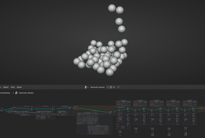
has only ten points. Let's say I want 100 points. If I increase the number of
points to 100 and hit play, you will notice that
the simulation will go haywire because when we
increase the number of points, we increase the
probability of error, and that will make the
simulation super unstable. So what is the
solution for that? Well, in our current simulation, we have 100 points
from the beginning. What if we figure
out a way to tell blender to not have 100
points from the beginning, but spawn them or
add them over time? That should lead to a
more stable simulation. How can we do that? Let's start with the first part
which is how to tell blender to spawn the particles over time?
That will be simple. All you need to do is to add a joint geometry
node and plug it as the first node in
the simulation zone. I will take the output
from the points node, technically from the store named attribute node and plug it
into the joint geometry node. What will happen now is
that blender will add more points each time
it runs the simulation. Or to be more precise, Blender will join the previous geometry with the new geometry. Next, I'm going to lower the
number of points to one, because if I don't do that,
blender will explode. It will start having 100 points, and every frame will
add another 100 point. You can easily see
how that will lead to having a crazy number
of points really fast, which will crash the software. When I change the number
of points to one, Blender will only add
one point every frame. Actually, that's still too much, and we'll need to
make a blender spawn a point maybe every 20 frames. But before we do that, if I hit play, as you can see, Blender is adding a
new point every frame, which is still too much, and it is still leading to the stimulation being unstable. The solution will be to
tell blender that T don't one point every frame. Maybe add one point every
ten frames or 20 frames. So how can we program
such a thing? I will start by adding
a same time node. This node will either give me the seconds value
or the frame am on. I will take the
frame and plug it into the count of
the points node. Now, at frame one, blender
will add one point. At frame two, Blender
will add two points, so I will have three
points and at frame three, Blender will add three points, so I will have six points total. That's not what I want. I
want to tell blender that a point every certain
number of frames. I will add a math node and I will set it to floored modulo. Floord modulo is just a fancy
way to say that this node will return the remainder of a division operation
by this value. This node will allow
us to specify how often we want blender
to add a new point. I will also add
another math node and I will set it to equal two, and the value should be zero. Here's the logic of
what's happening. Blender will take the number of the frame amon will then
divide it by this value, and if the remainder
is equal to zero. That means this equal
to condition is true, which means this node
will output one, so Blender will add one point. And if the remainder
is not equal to zero, that means this equal
two condition is false, which means this node
will output zero, so blender won't add any point. Want blender to add one
point over 20 frames. That's what I will get
if I type 20 here. Here's an example of
what will happen. Let's say I'm at frame 55. Blender will divide 55 by 20. The remainder of the
operation is 15. 15 is not equal to zero, which means this node
will output zero, and since this node is going to the counts of
the points node, that means blender
won't add any point. Now, let's say I'm at frame 60. Blender will divide 60 by 20. The remainder of the
operation is zero, zero is equal to zero, which means this
node will output one because this
condition is true now. That one will go to the
point count socket, and Blender will add one
point to the simulation. I think the logic should now be clear of what's happening. Now if I hit play, Blender will start adding
particles gradually, which is exactly what I want. The last thing I want to
do is to tell blender to spawn each point to
a different direction. I can do that by assigning a random initial velocity
vector to each point, which you can do easily by plugging a random
value node into the vector socket of the
store name attribute defining the initial velocity. And I's add the values to minus one minus 10
for the minimum, and 110 for the maximum. This is how we can make blender spawn the particles over time. Think the logic is super simple. In the next video, we will add fraction to our simulation.
15. Friction: Adding fraction.
An important part of any simulation is fraction. With no friction, the balls will just keep bouncing forever. That's why it is important
to figure out a way to tell blender to dampen
the simulation with time. And we actually touched
on this topic before, but what we will do in this
video is to make the process of changing the friction
a little bit easier. Now, this is our
entire note tree, and what I plan on
doing is the following. As you remember, in
the constraints, I have the velocity that is multiplied by minus one
depending on the axis. If I bring this value up
to something like -0.8, that will lead to more friction. What I want is to
change this value for all the different
multiplied nodes at once. This is simple. I will add a combined xy z node. I will input the same
value here, one, one minus one and plug that into the vector
of the multiply node. I didn't do anything fancy, I just replaced the value in the multiply node by this
combined x y z node. The reason I did that
is that now I can add a group input node and take the z axis and plug it
to the group input. Now if I go to the
modifier stab, you will see that I can
change the value from here. Also, it is important to note that I will only be
changing the value for the z axes because that's the socket plugged
into the group input. For the rest of the sockets,
they will stay one. This will make the
process of changing the values of
friction way easier. Now, I need to do the same thing for all the different
constraints. I will start by doing
it for the right wall, add a combined x Y Z node, and add a group input. I will move on to the left wall, add a combined x y zende
with the same values, and added group input. I will do the same thing also for the front wall right now. Lastly, I will do the same
thing for the back wall. S. And now I can control the
friction easily from here. I can also open the side bar by hitting n and the
geometry node editor, select one of the group inputs, and you can double click
to change the name of this property to
something like friction. For my simulation, I'm going to set the friction value to -0.9. Another way to add fraction
is by going back to the store named attribute
node defining the velocity, and if I add a vector math
node and set it to scale, I will be able to dampen the velocity on the
entire simulation. It's like a global friction
that will apply every frame. I can even add a group
input and plug it there, change its name to
global friction. I will set it to 0.99. The simulation will
lose velocity by a factor of 1% every frame. Also, it might be useful
to change the number of steps of the repeat zone
from the modifier step. That's why I will
also plug it into a group input node and call it, for example, sub steps, and I will set it to 20. Those are the values I
use for the promo render. Lastly, I will set my
frame rate to 120, so I will have a really
smooth frame rate, and my simulation will
be less prone to error. For the frame range, let's say I want a ten second render, which means my frame range
will be up to 1,200 frames. If I hit play, our simulation
is working smoothly. That's it, everyone
for this video. We technically
finished everything. In the next one, I
will show you how I created the final scene
and how to render it.
16. Final Overview: Hello again. On last time. This is the last video of building our own physics
engine in Blender. This video is a summary, slash a bird's eye view on everything that we did
up until this point. The first thing
I'll start with in this video is our notary, because currently it
is an absolute mess. If you decide to go back to
this project in the future, you will probably get lost in the C of all of these
different nodes. That's why I'll start by organizing and
labeling the notary, and then I will move
out to the summary. Okay, welcome back to Blender, and this is my entire not try, and it is a mess honestly. I'm going to hit
Control Space bar to maximize this editor. As you can see, there
are a lot of nodes, and especially in the future, it will be tough to
actually understand what's happening because we
didn't label our note try. What we will do in this
video, as I mentioned, is, first of all, to start by
organizing our note tree. I will go to the beginning
of the note try. I'm going to select
all of these nodes, hit Control G to create
a label around them, hit F two for a name,
and let's call it, for example, initial condition. Once we have our
initial condition, we enter the simulation zone. We have this joint geometry responsible for adding
points over time. After that, we define the acceleration using
this named attribute, and it is related to the
scale and this vector node. Make sure to select
the three of them. Hit Control G, F two for a name, and let's call
them acceleration. Next, you will have
the store named attribute responsible for
defining the velocity. Let's move it here. Same thing. Let's put all of these nodes on top of each other like
this by stacking them. Select all of these nodes, control G and F two for a name, and let's call it
velocity because we're defining the velocity
using these nodes. Next, we're updating
the position using the set position node, so stack the nodes
over each other. Select them, control G, F two, and let's call them
position update. After that, we enter
the repeat zone, which is responsible for compiling all the
different constraints. Let's put this node around here. Actually, I'll move
it up, but let's just try to find a solution in
this entire mess right here. Actually, to make
the whole process easier and to have more space, I will start organizing
these nodes from the end. I will have these nodes that are responsible for transforming
the points into the spheres, so I will select all of them, Control G to create a label, F two for a name,
and let's call it, for example, instancer. Move these back.
Move this also back. The less constraint
I have right here, it is the constraint
for the back wall. Let's select it entirely, which should be all
of these nodes. Let's organize them. First of all, you'll
have these nodes on top. I'm going to take Control G, and this is my condition. Let's organize these
nodes right here. Something like so. Maybe you will work. And then
elect all of these nodes, Control G, F two for a name, and let's call it
back wall strant. Next, you will have this. Do a similar thing,
select these, Control G and F two, and let's call it condition. Next, I will move
these nodes here. This one here, here,
these ones here. Select all of them. Control
G, F two for a name, and let's call them
front wall constraint. Now to the left wall constraint, all of these nodes, select these control
G F two condition. Next, is here, this one
here and this one here. Select the entire
note tree, control G, F two, left wall, constraint. Now to the right
wall constraint, Control G, F two condition, move these nodes here. Same thing for this one and
this one, then like so. Then select all of
them, control G, F two, right wall constraint. Lastly, the floor constraint, which are these nodes. We will do a similar thing. Select the control
G, F two condition. Move these ones here, for the position,
for the velocity, sorry, and select all of these. Control G F two
floor constraint. These are the
different constraints, and lastly, you will have
the collision system. Let's try to figure out a way
to organize all of these. I'm going to select all of
them and move everything down. I think this will be better. Let's put this one
here and maybe move the p zone and all of these nodes
slightly to the left, and then select all of
these Control G F two, and it's called it collision. This is my collision group. And bring this group input up, this slightly like this. And by doing this, we
organized our node tree. In the future, if
you go back to this, you will know exactly what
each group of nodes are doing. Because we labeled them. Also, when you take
this bird's eye view on the entire node tree, you start to see the logic
behind everything we did. As a final summary, here's the logic of
everything we built. First of all, we start by defining the initial conditions, how many points we have, when we want to spawn
points, and all of that. These points later will
enter the simulation zone. The first thing we
do here is to define the acceleration and then
define the velocity. Which we both use to update
the position of our points. Once we have this basic setup, we can start thinking about
different constraints. For our physics engine, there are two types of
constraints that we care about. The first one being
the collision, which is the collision between
the different spheres, and then the different
walls, which are the floor, the right and back wall, and the left and front wall. And at the end of the note tree, we use this instance
on points node to transform those points
into an actual geometry, which in our case happened
to be EUV sphere. And yet, This is our
entire physics engine. And yeah, that's
basically it for how you can build your own physics
engine in blender. Now you can create
a scene around the simulation and render
it however you want. Also, since shading and animation are beyond the
scope of the scores, and I wanted to keep the course concise and make it just
about geometry nodes. That's why I made a bonus free
video that you can watch, where I take you step by step
on how I created my render. You can watch either
from the link in the description or by
going to my website. The geometry node part and the shaving part are quite
different disciplines, and that's why it made
more sense to keep them as separate things since I take different approaches in
teaching both of them. Lastly, thank you for
tuning into this course. I hope you learned a lot. If you found this course useful, please leave us a good review that helps us make
better courses, and you can still check the
rest of my courses here. Thank you very much,
and I'll see you or.
 Yassine Larayedh, VFX Artist