AUTODESK INVENTOR 101 | CAD & FEM for Beginners

1. Introduction: Welcome to the inventor course for beginners. Thank you for choosing this course. In this course, you will find an introduction to the basics of the great cat program inventor from Autodesk and learn in particular the cat design in detail. As an engineer, I will show you step-by-step my knowledge from my studies and professional practice so that you can achieve optimal learning success with theoretical basics on the one hand. But above all, with practical examples. On the other hand. After a theoretical introduction, this course includes many practical design project to learn designing the program from scratch and with inventory from Autodesk. As with other CAD programs, you can not only design, rather of this program combines and links several engineering disciplines such as cat, computer aided design, and femme element method. In one platform. Within renter, you cannot only create components or assemblies, but also perform simulations and animations, as well as create renderings. The main focus of this course is on design within renter. That means the cat part of the program, but the other functions will not be neglected, don't worry. As already mentioned, the abbreviation cat stands for computer aided design. What is cats software anyway? Cats software is used to virtually create or edit three-dimensional objects, starting with simple individual parts through complex parts to an entire assemblies that can be virtually assembled. This course, specially designed for beginners, you will learn how the inventorial environment is structured and how to make the most of its features to create three-dimensional objects. It's project of the course can be followed step-by-step in one-by-one in order to get an easy introduction to the material and to become more familiar with the multiple functions of the program. Each lesson. In a nutshell, this means that you can learn the following in detail in this course. Find your way around the inventor program quickly and confidently. Master all the important functions of inventory quickly and confidently. To learn the basics of cat design and the different ways of working methods. Get to know 2D sketching and 3D object creation. Create individual parts and assemblies, render and animate in the ritual parts and assemblies. Simulates in your ritual parts and assemblies. That means apply loads and display stresses and strains. Fem simulations, learn the environment of technical drawings and create technical drawings. It is best to stay in the order that the course provides as lessons build on each other. If you do not understand any ritual functions or commands right away, or miss the explanation for our function, just stick with it. The course is structured in such a way that all important and basic functions are explained sufficiently and in an intuitive way. Therefore, explanations in the chapters may overlap or certain functions may not be covered in detail until a later chapter. 2. The CAD software "Inventor": The professional cat program in Venter from Autodesk offers a clear and simple user interface, but it also has its price. A licensed currently costs about 350 euro per month annually, about €2,900. If you buy a license for a longer period, you can save a little. Pupils and students have the possibility to get a license for the duration of their studies. All others can test the program at least for 30 days, free of charge. In its full extent, it is no longer possible to buy the software directly. There is only the possibility to subscribe to the software for a certain period of time. With a subscription, inventor can then be installed on up to three computers. However, it can only be used on one computer at a time and only with the purchases login data. The structure of the design features is relatively identical for all common cat programs used by engineers or technicians in their daily work. There is a basic selection of professional cat programs. In addition to Inventor, the best-known, our SolidWorks Catia, Solid Edge pro engineer, also known as Creo, and probably the best known of them all out to get. There are basically no major differences in the prices. So these programs are usually only worthwhile for professional users and self-employed people. And now we're ready to get started. Before we get to the basics of cat design, we will make general program settings and familiarize ourselves with the program interface and functions. 3. Preparation: First steps with the program and general settings: When we start the program for the first time, we are initially presented with three windows and three menu bars. In the menu bar, get started. We find standard options, such as creating a new file or opening an already created file. In addition, we can work through tutorials, see what is new in an updated version of inventor and request or look up help. In the Tools menu bar, we can use the application options button to make initial settings for the program or reactivate existing settings. With the help of B settings, the program can be individualized to some extent. E.g. the background color can be set in the colors section. I prefer the white presentation layout or graphic settings, depending on the hardware can be made in the hardware menu tap. Here we have to choose between quality of display or performance depending on the equipment of the PC. In the sketch menu, we activate two functions, namely grid lines and snap to grid. That grid is displayed to us when sketching in the 2D environment. And we can select the grid points more easily with the cursor. However, this setting is really just a matter of taste. At last, we want to make setting for the units at file with a click on configure default template, we can change this to millimeters and set the drawing standard to all other settings are not needed for the time being. They are much too special for the start and can be left at the default values. We are now still in the start window of the program in which there are still the three sections, new projects and recent documents. These are relatively self-explanatory. In a recent documents, you will see the most recently used files after the creation of the first fires. In the new section, we can choose between the creation of a single-part part and assembly. Assembly, a technical drawing drawing, as well as a presentation. If you have never worked with a cat program. Before, you may wonder what the difference is between a single part and an assembly and why a distinction is made here. Think of it very simply, just like in the real world, in the virtual environment of a cat program, every more complex part is assembled from several individual parts. A car, e.g. has thousands of individual parts from the steering wheel to the smallest bolts. Each of these parts is an independent individual part that when assembled as a whole, results in an assembly, the car. And the cat program and assembly is therefore made up of all the individual parts. Just as in real assembly. With drawing, a technical drawing and in the ritual part with views, dimensions, and all the necessary information is described on a sheet of paper in 2D in such a way that it can be manufactured in accompanied by an employee. And assembly can also be described with a technical drawing. Since we want to start designing our first still very simple part as soon as possible. We therefore now first select the creation of a new single part. By the way, single-part assembly and technical drawing each have different file extensions. In this case, the extension IPT stands for pot. That means in the ritual parts, that extension I am for assembly and the extension D, W, G for drawing. That means technical drawings. A look at these extensions will help you to identify what you're dealing with in a file. Then we get to the actual program environment of inventor, in this case, to the environment for individual parts. By the way, we can return to the initial window by clicking on the small box in the bottom bar. In the next chapter, we will take a first look at the program environment and functions of AutoDesk Inventor. 4. First overview: Program environment and Functions: Let's first take a look at the program environment in the menu boss located in the upper inside areas. The menu bars in the upper area are different for each of the four environments, part assembly, drawing and presentation. While there are always some taps that appear in several or all environments, such as 3D model or sketch. There are generally different types and functions depending on each environment. We will learn what the differences are during the course. So now we are in the environment part. At the top-left file allows you to open, save or export files and other basic commands. The selection tabs on the side of file can be used to switch between the individual sub menus for the features in their respective environment. In this first section part, we will first deal with the design features for a single part. There are ten different tabs here. 3d model, sketch, annotate, inspect tools, manage view environments, get started and collaborate. The 3D model menu tab, you will find all the functions that are necessary for creating or editing a three-dimensional object. In the create section, you will find all the functions for creating a 3D part. In the Modify section, you will find all the functions for editing 3D part. What these functions can do and how to use them. We will learn in detail and step-by-step during the course. In this chapter, we first want to get an overview. The shape generator can be used to create an optimized components structure based on a load situation. In the work features, we find all the tools for construction. That means x is Plains, points and coordinate systems. In the pattern area, a pattern command can be used to save a lot of time and effort during construction. The two areas create free form and surface, are intended for the free form or surface modeling mode of operation. However, we will not cover this advanced cat the way of working in this beginner's course. It is also only necessary for very complex parts. With the last two points, simulation and convert. On the one hand, a femme load analysis can be started or a sheet metal part can be designed. By the way, with the small error on the far right. This bar can be customized in each of the menu tabs. That means needed or not needed sections can be shown or hidden. For us, e.g. primitive is interesting with which simple bodies, such as a cube can be created directly in the function measure, with which you can measure something in the 3D environment. In exchange, we hide, explore, and create free form. You are also welcome to take a look at the other possible sections. In the next section, sketch, which is intended for 2D sketches, we first find, create, modify, and pattern again. Here, lines, circles, or other 2D geometries can be created or modified. If you do not have any previous knowledge, you must mentally divide the cat program and the design of an individual part into a two-dimensional and three-dimensional area. You start with a 2D sketch and then create that 3D body from it. But more about that later. In the annotate menu tap tolerances, dimensions, surface specifications, remarks can be applied directly to the 3D component as an annotation. However, this is normally not absolutely necessary and is usually denoted on an engineering drawing. However, applying these annotations directly to the 3D part can have advantages on the 3D model is transferred to manufacturing in addition to a drawing, a tolerance analysis can also be started in this area. In the menu tabs, inspect and tools, you will find again, the general measuring function, as well as the possibility to start various analysis. The possibility to change the material or the appearance of a part, as well as a few more commands that are rather unimportant for us for the time being, we will skip the Manage menu tap since its content, it's also unimportant for this beginner's course. Important however, is to tap you with which the display of our components can be controlled. Here, in addition to the general component display, which will style the focus or shadow, as well as a background can be displayed. But more about this later. The last important areas to tap environment. In this tab, you can switch to the other environments of inventor. In addition to the cat design, inventor can also be used to perform an FEM load simulation with stress analysis or to create an animation and rendering with inventors to do. Tolerance analysis can also be performed, and there is also a specific environment for creating castings and more. For us, we already mentioned possibility of sheet metal design with Convert to sheet metal is still important. The last two menu tabs get started and collaborate are very self-explanatory and contain rather general commands. Feel free to click through here if needed. Don't be afraid of the multitude of elements and features. The course of the course, we will get to know the individual elements step-by-step and in detail using practical examples. If we now look at the drawing lay layer area, we find the part browser of the construction file in the left area. If it is not displayed or if you have closed it by mistake, click on the small plus symbol and select the model browser. This part, or modal browser, contains all views, as well as the origin, the planes, and the axis of a file. However, the main function of this part browser is to list the created sketches, construction elements in order to activate, deactivate, or edit them with a right-click on them. We will see later how this works. It is also very good if you get into the habit of naming the individual components and possibly sketches and layers right from the start in order to find your way around the complex construction more easily later, simply double-click on the element and enter a new name. In the narrow bar above this part browser, you will once again find general functions such as open, safe, undo, or redo, and settings for selecting elements or features, as well as settings for the material and the appearance. It may be that this bar is also displayed at the top with a click on the small error on the far right. You can change the display position if necessary. In the upper-right area is the orbit cube. Here you can select views of the current construction and rotate the drawing environment encoding the object. Rotation of the drawing environment is also possible with the shift pressed while moving the mouse. Shifting is possible with a mouse wheel pressed and the mouse movement. The zoom function is performed as usual by turning the mouse wheel, by right-clicking on the drawing environment, we can access the Quick Selection Menu, which can be used to quickly execute a variety of commands. In the lower part of the drawing environment, we can switch between several open fires. The bar on the right side below the orbit cube also gives us the option to move or rotate the environment, as well as the look at command, which makes it very easy to look vertically at a selected area of a component. In addition, and navigation wheel can be activated in this bar, which is then permanently displayed and serves as a kind of quick selection menu. Here, you can also choose between different designs. Very well. After this chapter, we can find our way around the program environment relatively easily and can start with the next chapter. Has already mentioned common cat programs work in a very identical way. We would now like to look at this way of working in detail in the following. 5. 2D sketching environment: Each 3D component must first be started as a 2D sketch. This is where we define the floor plan of the object, so to speak. You mentioned that you are taking a look at the top of a simple three-dimensional object, e.g. what do you see in a cylinder when you look at it from above at a perfect right angle to the axis, correct? Two-dimensional circle, nothing else. It is exactly from this 2D shape that the cylinder, analogous to all other elements, is also created in the cat program. It is exactly this circle geometry that we have to draw for this object, e.g. first step, the three-dimensional shape is then obtained by furlough command steps for the 2D sketch, e.g. also the top surface of an object or a side surface, or also a partial surface comes into question. Here you need some spatial imagination. For each 3D part. As we said, we must first make a two-dimensional sketch. We will look at how to create a 2D sketch in detail in this chapter. At the beginning of a sketch in the 3D model area. Alternatively, also in sketch. Select the start to the sketch command. Then we are shown the planes of the coordinate system. And we have to decide for a plane of the three-dimensional space on which we want to draw our 2D sketch. In our example, we want to look from above at the circular surface or top surface. So we should choose the x z plane. That is the plane that the x and set X is form. Which plane you choose is only important for the alignment of the views. The program then opens the selected sketching plane for us. As you will notice, the sketch menu bar also opens automatically in the upper area where you can find all the commands. A verity of basic drawing elements are now available for creating the geometry of a 2D sketch by selecting a line, e.g. a. Geometry can be formed from line shaped elements. Let's try this out. To do this, simply click on any point, e.g. on the center of the coordinate system and start drawing by clicking and dragging with your mouse. With another click, you create the line. If you then want to continue drawing directly after this line, simply continue drawing. If not, use the Escape key and start again at a different position. The drawing should correspond, e.g. to the cross-section of the desired 3D object, or in the case of simple objects, to the upper surface or cross-sectional area of the object. Enter the desired dimensions using the keyboard. You can switch between dimension and angle using the Tab key. You can also draw freely and use that this plague values as a guide or add or change the dimensions and angles later, the small symbols that are displayed for a rectangle, e.g. or the constraints or dependencies of the respective lines. We will take a closer look at these in a moment. Besides a line, you can also create the circle and ellipse a free form curve, an arc on oblong hole or a rectangle. Let's just drive that out one after the other as well. You will also find in the Create menu a point where we use arcs and several other elements. It is best to simply try out all elements at least once. To do this, simply pause briefly and start independently in the sketching environment of the cat program, it is best to use this approach throughout the course. This is the most effective way to learn. Another tip about the prefabricated geometry elements such as rectangle or so-called. When drawing, you will notice that the rectangle, e.g. starts from a corner. However, if you want the rectangle to spend from the center, you can also use the drop-down menu at the rectangle to select a center rectangle or also two-point rectangle. With the circle. You can, if desired, also create a tangential circle instead of a center circle, e.g. in the Modify area, we can perform various operations to modify a sketch. First, let's take a look at the move, copy, scale and stretch commands. These work in a very similar way, but of course, each does something different. Let's try the commands on the example of a rectangle. The way it works is as follows. First, select the command e.g. move, then select the cursor, select in the window. And the next step, select the rectangle or the new ritual lines, or another geometry element with the mouse. Then select the base point cursor in the command window and deep define a reference point on the drawing plane. Now, when we move our mouse, we can see how the, how to move the part based on the reference point. You can then place the rectangle in the desired position with one-click. For copy, scale and stretch. This works as said, in an identical way. For rotate. We don't need a base point, but I have to enter an angle for the rotation. Trim and extend can be used to shorten or lengthen a line segment. Split can be used to split the line into two lines at the closest point. And with offset, you can create an identical geometry element with a distance to the original one. Here you can perform relatively basic drawing operations. We will get to know the menu area pattern later in the course. Before we conclude this chapter as promised, let's get to know the role of constraints. You can use these in the 2D sketching environment and use them to create constraints between individual geometric elements. This is sometimes but not always, necessary or helpful. By the way, in this area, you will also find that they mentioned function for creating dimensions. We will now take a closer look at the most important constraints. Let's start with the horizontal and vertical constraints. Let's assume that we try to draw a rectangle freehand. And we get a polygon whose lines unfortunately do not represent a rectangle. By selecting the horizontal condition, we can create two perfectly horizontal lines by clicking the top and bottom lines. In an identical way, we apply the vertical condition to the lateral lines and end up with a rectangle. As you can see, these conditions are displayed to us as small icons next to the respective line and are also already suggested when creating a sketch. In the bar at the bottom, you can also hide the display of these conditions. In addition, you can use snap to grid to set whether the cursor should snap to the grid points when drawing. That means whether it should remain attached to the grid points for easier sketching or not. Back to the constraints with the relation concentric to circle structures can be said concentric to each other. E.g. let's draw a large circle and a slightly smaller one. We want to get two concentric circles. That means two circles are the centers are congruent. We achieved this by selecting the appropriate dependency and the two circles, the two constraints perpendicular and parallel, are relatively self-explanatory. Nevertheless, let's look at a small example with two lines each. For the function perpendicular, we draw the following two lines. By selecting the condition and selecting the lines we get as a result, two lines that are perpendicular to each other. For parallel, we draw two more lines. And by selecting the condition, we get to perfectly parallel lines. We use the constraints coincident, that means congruent and co-linear whenever we want to connect two points or bring a line into linear dependency with another line of another element. To illustrate, let's draw a rectangle and two lines. We want to connect the first line to a vertex of the rectangle and make the second line colinear with the other line. The way you can also apply multiple constraints, e.g. we could also still apply the constraint horizontally to align that already has another constraint except vertically. Let's take a look at the tangent condition as the name and the small picture already indicate. We can use this to set a line tangent to a circle, e.g. let's try it out. First, draw the circle, then align, and then apply the condition. Just try the two constraints fixed and equal wants yourself. You can't go wrong and the name is relatively self-explanatory. The fixed constraint simply fixes an element in the place in the drawing layer. And equal ensures that the same dimensioning exists between elements. With symmetric, you can set two elements, e.g. two lines symmetrically to a third line, the symmetry axis. Simply draw three lines. Select the first line, the second line, and finally third line. And the two outer lines are aligned axes symmetrically to the middle one. With the command image. We could insert an image into the drawing environment, e.g. if we simply want to trace a geometry. To conclude this first 2D sketching exercises, please draw another circle in a new file, which you can then provide with fishes dimensions using the dimension function, e.g. select a diameter of 50 millimeter. Simply draw the circle and select that. The dimension tool. There are two ways with dimensions, both of which lead, lead to the goal. You can draw a circle with. The dimensions are already correct by entering the values using your keyboard while drawing. Use the Tab key to switch between the individual fields for entering dimensions. Alternatively, you can draw any circle and then change the dimensions. You can also use this command to dimension the distance between two lines. To do this, simply click first on the first line and then on the second line whose distance you want to dimension. You can exit the 2D sketching mode with the green check mark in the upper menu bar. The program then switches back to the 3D environment and chose us our sketch as a profile on the selected plane. To create a three-dimensional object, it is important that the 2D sketch is completely closed and has no gaps. By the way, with a double-click on your mouse wheel, you can fit an object into the current view. This is very helpful if you ever find yourself very far away in virtual space and can no longer see an object. In the next chapter, we will create a three-dimensional object from the 2D sketch we made. Very good, you're making good progress. Soon. We will already get to the first real design project. 6. 3D object environment: In this chapter, we would now like to create a 3D object from the previously sketched to the surface. To do this, we will use the functions from the create section in the 3D model area to create a cylinder be used probably the most needed function from this menu, we use the command extrude. This function represents a so-called extrusion command and other CAD programs, you will therefore often find the term extrusion or extrude linear. Now, simply select the function and the profile is normally already extruded automatically. If not, simply click on the profile, drag the displayed orange arrow with your mouse in the possible range of motion and change the dimensions of the 3D objects in this way. Alternatively, you can also enter the desired dimension right away and confirm with enter in the window that opens when you select the Extrude command. And it's called properties, you can select or deselect the profile and also specify the direction of the extrusion. That means to which side it should be extruded or whether it should be extruded symmetrically in two directions from the sketch plane, e.g. under Advanced Properties, you will find the option to make the object conical. Before we deal with the other commands from the Create menu, we will use the constructed cylinder to first get to know the most important commands from the Modify section. We use this section whenever we want to modify and already constructed object. E.g. we can use the filter function to round one or more edges. Simply select the function and select one or more edges. Appears again, which we used as with the extrude command in the Properties window. We can then change further options. In an analogous way, we can create a chamfer with chamfer. Another important command is shell. With the help of this command, you can easily hollow out an object. That means create a thin-walled 3D object. Select the command and the face of the cylinder and enter a wall thickness or use the arrow. Pretty simple, isn't it? The other commands are applied just as simply. Withhold. A whole can be created with thread, a thread with combine, you can unite solids with split. You can split them again. We will look at these commands in more detail later. With the draft command, you can quickly create a slope or in-kind. Simply select two phases of a 3D object and enter a slope angle. With thicken offset, you can strengthen a face with additional material. And with delete face. You can delete the face. Now that we know the most important commands from this section, Let's turn once again to the Create menu. Besides extrude, we find here the important commands revolve, sweep, loft, and more. The explanations and sample images of the software are very clear and helpful here. And already give us the first hint of what these commands can do. We will look at how to use them in more detail in the next chapter. As this is related to how CAD design works. By the way, in, in renter for some elements, it is also possible to shorten the process from 2D sketch to 3D object by combining both steps, which can definitely save some time. E.g. in the Primitives section of 3D model, we can immediately construct a cube root, a cylinder or a sphere, and other elements with the respective command. Simply select the command, sketch the footprint onto a plane of the 3D space and extrude the element. Now on to the next chapter. 7. CAD Design working methods: As already briefly mentioned in the previous chapter, there are different approaches to the design of 3D objects. One possible approach to this sign is e.g. to design as the actual machining, e.g. a. Milling or turning of the starting material, the so-called semi-finished part, would proceed. In the cat program, you first create the raw material, in this case the cube root material, and then work successively further steps using cutouts, holds, floods, and other design features were Chile, so that you get the final element. That's why this method of design is called subtractive. You reduce the initial material through individual processing steps until you get the desired object. But there are also other approaches, such as the additive method. Here, the cat model, or even the real object, as is the case with 3D printing, is pulled up element by element. We will take a look at how this works in concrete terms in a moment. We will first deal with the classic subtractive approach. The next steps, we want to make a hole and the cutout in rectangular form in a simple cube. I have already prepared the cube. The dimension is e.g. 50 millimeter in all directions. To create the whole, we can use the whole function from the Modify section. Simply select the command and the surface on which you would place the drill in reality. Then select two edges and n two-dimensions to determine the position of the hole on the surface. In the Options window that appears, you can then select the type of hole, that dimension of the whole end specific hold parameters. E.g. we select a simple so-called through hole with a diameter of ten millimeter. We can also create threads here, but more about that later. For the cut-out, we first need to create a 2D sketch of the geometry. Again. To do this, click on Start to D sketch and select e.g. the upper surface of the cuboid. Since we want to bring the section into the ID from top to bottom, place a rectangle on the surface and the area of the cube with a click and enter dimension of ten millimeter each. Confirm with Enter. Then we define the position of the rectangle on the surface using the sketch dimension or dimension function. Since we are in two-dimensional space, that means sketching on a parallel of the exit plane. We need an x and the set dimension to finally define the sketch completely entered the desired dimensions, e.g. five millimeter each from the left and upper edge of the cubit. Now the rectangular is completely dimensions. As you may have noticed, the profile has turned blue. This indicates that all degrees of freedom are fully constraint. That means position of the profile and the plane is fully defined by dimensions and constraints and cannot simply move by itself in later editing steps. A complete dimensioning and a fully defined sketch are very important for good results. Always pay attention to them. After we have finished the sketch, we can create the section using the extrude function, e.g. the cut-out should go completely through the part. The extrude function can now be used to both the remove and add material from the created sketch. So you can use extrude and the design for a subtractive approach, but also for the additive way of working. To make the difference between the two working methods clear. We will now design our first very simple pod, which could serve as an assembly component for a machine, e.g. first with additive working method and then with subtractive working method. By the way, it doesn't matter which method you choose. They both lead to the goal. The only difference here is in terms of effort and time required. For the additive method, we simply draw the cross section of the pod. In this case, we can even do it in one step. Of course, we could also split apart into its rectangular bodies. And london, London map body by body, which would be more like the actual additive way. But that would be very cumbersome. So in 2D mode, we first draw the cross section of the part on the plane of the coordinate system. Start by selecting a new sketch and the plane. By the way, you can also right-click on the desired plane and the pod browser and then select Create Sketch. We then draw the first line is shown. Complete the profile with the following lines and dimensions. Simply trace them. Then complete the cross-section profile with additional lines as follows. Then you can leave the 2D sketching environment and thus switch to 3D mode, select the extrude function and create a three-dimensional body from the 2D cross-section using a dragging movement in the direction of the displayed arrow, enter a dimension of ten millimeter with the help of the keyboard. That's it. Finally, we create three holds for mounting. For this, we use the whole command. Now we would like to use the subtractive design method for the same part for illustration purposes. To do this, we draw a rectangle with the dimensions 50 millimeter and 30 millimeter in 2D sketch mode. And create a cube root with 20 millimeter using the extrude function. With us virtually first create the starting material, the so-called semi-finished product, from which the pod will be punched out, cut out, or move out. In reality, e.g. then we draw the cutouts in the solid material. To do this, we first create a 2D sketch on the upper, alternatively, of course, the lower surface. First sketch the upper half of the cut-out for the geometry of the part using lines. Make sure that surfaces are created. That is, that you also connect the profiles at the edges. And then the bottom half. We can also simply create a rectangle for this. Instead of using Alliance, we draw the negative of the part into the solid, so to speak. We can also draw the geometries for the holes in this sketch at the same time to execute them as a cutout instead of using the whole command and save ourselves a step this way. Then you can again use the extrude function to cut out the drawn faces from the solid. Two approaches for an identical solution. One quite simple, the other a bit more elaborate. Now let's look at a few more possible ways of working. In addition to the extrude function, there are a few other functions in the create section that we would like to take a brief look at in this chapter. First, there is the Revolve command. You can use this whenever you want to construct a part with a rotation axis, e.g. apart, that in reality would be machined by turning. To do this, simply draw a cross-section on one of the planes, e.g. on the exit plane or x y plane. Why these planes? Because we want to use x as our axis of rotation. But you could also use the y set plane and then use y or set as your axis of rotation. Let's take a closer look. Feel free to draw along with it. E.g. we will create the following basic profile of a bolt in the 2D environment, we need to draw one half of the cross-section of the 3D body. After finishing the sketch and selecting the Revolve command, we must first define our rotation axis, in our case, the x-axis. As you can see, the software then creates the solid by entering a number of degrees, you can define the range of rotation. Of course, such a bulge could also be treated using several sketches in an additive manner using the extrude function. Just think for a moment how that would work in this case. However, the way via rotation is usually much faster and more elegant for such turned pot. This is what I meant when I mentioned that there are several ways of working, even for one in the same pot, depending on the part. These are faster, slower or her simple or cumbersome, but usually all lead to the goal. The sweep command is always useful when you want to create the part that follows a slightly more complex path. Let's take a look at how to understand this. For the sleep command, you always need a 2D sketch, cross-section profile, and the path that is simply a line or an arc or spline or free form curve, e.g. let's create a spline by selecting the command in a 2D sketch on the x, y plane and drawing several points as you like. But make sure that the end point or start point is the coordinate center. The more points, the more detailed the contour will be. For the cross-section profile, we now have to change the plane. To do this, we close the sketch and start a new sketch. On the y set plane. We draw e.g. a. Circle or a rectangle and select the endpoint of the previously drawn deposited profile in the x y plane. Then when we finish the sketch in 3D mode, we can run the sweep command and would normally have to select profile first and then the path. However, the program already creates the solid automatically. In the Properties window, we could still make various settings, e.g. change the alignment. The last important command from this section and for this chapter is loft. With loft, simply put, you can have two surfaces connected to each other in 3D space. Let's try it out. We will draw a profile in the x, y plane, e.g. a. Rectangle or any other shape. We first create a new plane parallel to the x-y plane with an offset to it. Right-clicking on the x y plane and selecting offset plane makes this very easy. We then drag the arrow or enter a dimension with a keyboard. On this new plane, we draw the second surface for our project in the next step, e.g. a, slightly larger rectangle. The centers should be congruent. Then we finish the sketch and select the loft function and the two sketch surfaces. The program then joins the two surfaces to form a 3D solid. With the settings, we could still control this process in detail. Where are we good? So much for the approach and working methods in CAD design. We can successfully check off this chapter and move on to the next one. And the following, we will take a closer look at the difference between a single part and an assembly. 8. Individual parts vs. assemblies (constraints & joints): As in the real-world, you can also will actually assemble a component or assembly from several individual parts in the cat environment to design a complex machine or other complex assembly. One first designs the individual parts of this complex part and then virtually assembles these individual parts in the software. To do this, you use mates, connections, or relationships. In Inventor, there is also the possibility to create joints. But more about that later. In Inventor, you create the parts and the assembly in a separate environment. When you have finished creating the new ritual parts, you insert all the individual parts of an assembly into the file of the Assembly and then connect them in the assembly environment, e.g. to a machine or simply set to an assembly. Each individual part has its own origin and its own folder in the pot browser of the assembly. The assembly itself also has its own origin. I'll look at programs are structured somewhat differently here. And e.g. everything can be created and joined together in one environment. So how does this work for an assembly, you must first create all the parts in the part environment. When you have finished designing the first part, e.g. such as simple turned part, which you can create yourself using the following dimensions. You simply create a second new part in a new file. We could e.g. draw another such profile for a second term part, which we then create again using the revolve function. Then you create an assembly file. The two individual parts are then inserted into this assembly using Place. Click on the drawing layer to insert the part. If you want to insert it again, simply click a second time. If not, end the process with the escape key. Alternatively, you can create a new pod directly in an assembly. To do this, use the create command from the assembly menu in an assembly. This is often very helpful since the first component remains as a reference and thus the dimensions for the new part can be very easily drawn, are determined to fit exactly. This would then work as follows For our second single part. By the way, whether you want to create the new single-part directly in the assembly, or whether you created in the single-part environment, is a matter of taste and varies depending on the user and the way of working. Let's now take a look at the assembly of these two individual parts. We can move the tube inserted in the ritual parts freely in space. So we need to link the two individual parts in the next step to define the positions and the range of motion in three-dimensional space. Here we need the assembly menu. In Inventor, you have two possibilities to link parts with each other. On the one hand, you can work with constraints, as in many other CAD programs. With these, the movement range of individual parts is restricted. We already know this from the 2D sketch environment. It works similarly in 3D mode, e.g. you can create the distance link, or e.g. a. Concentric constraint between two parts to get an assembled and fixed positioned assembly. On the other hand, you can work with joints instead of restrictions, one creates a defined range of motion through a joint. An example in a hinge joint of a garden gate, e.g. only one rotation around one axis is allowed. All other so-called degrees of freedom are blocked. Thus, no other movement can be executed. First, the method of constraints or restrictions. This is also used by default and other CAD programs and is therefore generally a bit more common. To link our two example parts, we choose a concentric constraint, which in this case is called insert. Simply select, then select the axis of the two individual parts to be linked. And the two parts are joined together and are now firmly connected. The restriction is then displayed to us in the pot browser in the folder of the ritual part. We can also edit this here with a right-click on edit, e.g. we can add an offset if we want the distance between the two parts or change the alignment. There are also other constraints are soluble, namely made angle, tangent and symmetry. With mate, you can make two surfaces congruent with each other. Simply select one face of the first part and one phase of the second part. These two surfaces will then be congruent with each other. A movement in the plane is still possible. With tangent, you can connect two elements tangentially and with angle, you can create an angular relationship between two elements. Based on the name you can already derived the function very well. 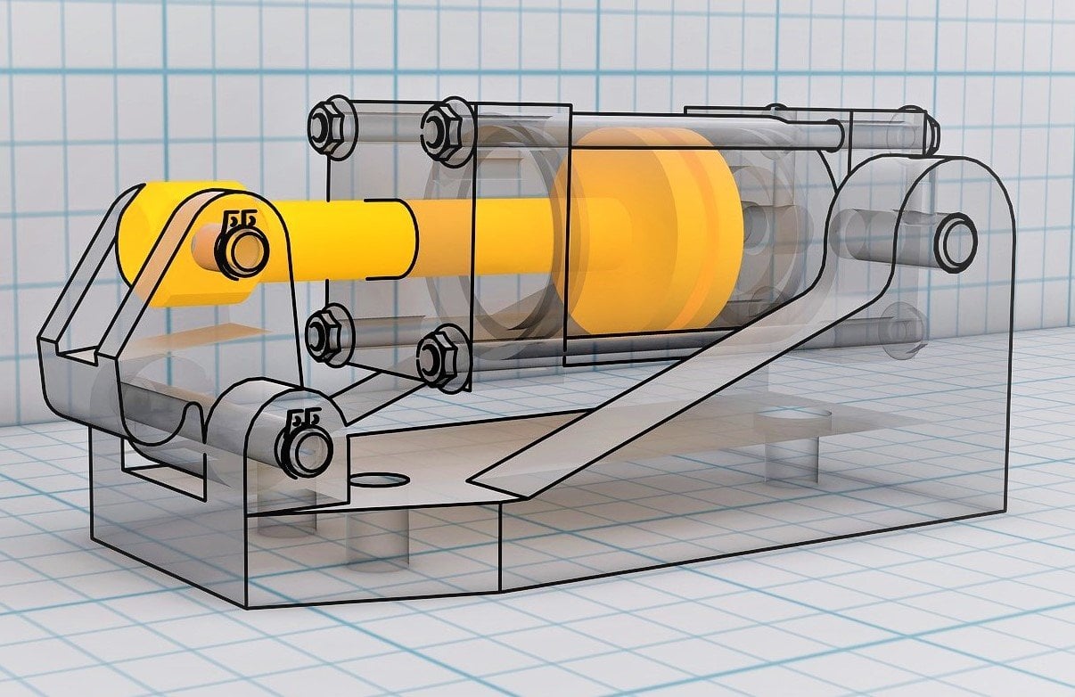The goal is to link the individual parts. Realistically, that means to link a bolt, e.g. concentric Kelly and the rigidly with a borehole of an assembly pod or e.g. to link a piston of a lifting cylinder so that it is guided linearly and has to stop points. However, our two joint individual parts can now still be moved freely in the assembly, since the reference to the origin of the assembly is still missing, the easiest way is to fix one of the two individual parts at the origin. We do this with the ground and root command from the Assemble menu section in the productivity area, simply select the item and command and then enable ground at origin and optionally create origin flush constraints. Then the part is moved to the origin of the assembly and fixed there. If the option create origin flush constraints is activated. Three constraints are created for the fixation. If not, the part is fixed without constraints. The advantage of the constraints is you can edit them later if you want to. Another advantage is that you can animate constraints in the animation environment Inventor's Studio with one-click. That means you can play and record a movement. This is not possible with joints. By the way, you can also drag a single part into an assembly. Simply select the part and drag it into the assembly. If it is the first part of the assembly, it will be aligned and fixed based on the origin. So you don't have to use the ground at origin command. The next part that you drag into the assembly is then initially free to move. Again. As already mentioned, inventor also offers the possibility to use joints for these connections are the assembly of single parts to an assembly in the menu assemble. We first select the command joint. Then we have to perform two steps. On the one hand, define the positions of the joint origins. E.g. select the points on the surfaces we want to link. And on the other hand, define the range of motion using the joint. Let's try a few possibilities. On the one hand, we could select these two joint origins on these surfaces and create e.g. a. Rigid link with rigid. By the way, when selecting the relationship, a short animation of the possible range of motion is played, which I personally find very helpful. A really great feature which makes this program very descriptive. On the other hand, we could allow a rotation around the y-axis with rotational, with slider, we can allow a movement along the x-axis. And with cylindrical, both a movement along the y-axis and the rotation around this axis. With Planner, the component can move linearly in a plane and rotate around an axis. Very interesting is also the function ball, which creates a ball and socket joint in the field gap, an offset. That means the distance between the joint origins can be selected with the buttons at align. The alignment of the joint can be changed or murmured at the surface. If we switch to the limits, step, further settings can be made, such as determining a start and end position. If we now select the motion type cylindrical, e.g. we see that we can only move the component and the defined degrees of freedom. The joint also appears in the folder of the linked component in the part browser and can be deleted, suppressed, or otherwise edited by right-clicking on it. By the way, if no range of motion is desired, the relationship Richard can usually simply be selected. The advantage of joints is that often the same can be achieved with a few clicks as with the constraints. So they are two ways of working, both of which have advantages and disadvantages. E.g. if you plan to create a dynamic simulation, use joints. If you want to create an animation, you should use constraints because unlike joints, you can animate them with a one-click. Perfect. In this lesson, we have learned how to create multiple parts and inventor and link them together or assemble them virtually. In the next lesson, we will take a look at different views and representations. Then we have learned all the important basics. And finally, get down to the Great and practical design projects. 9. Views and representations: In this lesson, we will briefly look at the possible views and representations in Inventor. The basic views can be found on the left in the pot browser, in the folder view. In this folder, we can choose between top, front, right, isometric. If you want to look at the specific surface, we can select the surface and the small menu bar on the right side with the function, look at a line to the surface will then be displayed vertically from above. With the function assumed window. Also from this bar, we can enlarge a defined area. To do this, we simply drag a small window around the desired area. In the menu tab view. In the upper area, there is the selection menu visual style, with which we can change the display of our components. On the far left, at object visibility, we can generally define which elements, such as layers and access should be displayed or not. Here we can also create a section view. We do this with the command section view from the section with the polity at view. We can display a half, quarter or three-quarters of the part and thereby look inside. Just think of it as cutting a cake and looking inside. For a quarter view, we select the command and the first plane, e.g. the y center plane. Then click on the small arrow and select the second plane, e.g. the x, y plane. Now the section view is created by the way, for our half cut, you only need to select one layer. You can also set an offset using the arrow or the keyboard with n section view from the drop-down menu, you can end the section view. Finally, we will get to know a few useful displays from the inspect menu. Using the section command, we can also display and even analyze the cross-section of a component or assembly. After selecting the function, we have to choose the plane in which we want to cut the part. Alternatively, we can also select the surface, e.g. we select the y set plane. The park will then be cut. In this plane. We can now either confirm or move the cut surface using the arrow or by entering our dimension. After confirming the section view appears in the Analysis menu folder on the left of the pod browser, where we can edit or delete it with the right-click. In the Inspect menu. You will also find, analyse this functions such as the zebra analysis. With the help of this, you can check transitions between surfaces by means of black and white stripes projected onto the surface. And e.g. examine the surface of an aircraft wing for its surface continuity or smoothness. This is so important for the flow resistance, e.g. to conclude this chapter, Let's take a look at the pop browser on the left. Here, the individual design steps are shown in chronological order and refund the generated features, such as Sketch, extrusion and so on, one after the other, depending on the design. The great thing now is that with this part browser, the design can be reproduced relatively easily. You can also return to a specific point in the design by simply placing the branch with the red dot called end of part, in front of a specific construction feature. The program then chose the part with all design steps only up to this point. By right-clicking on the individual design steps. You can also edit the respective steps, e.g. a. 2d sketch or change the properties of an extrusion. This bar is also very helpful in order not to lose the overall view. Especially with more complex designs. Especially if you're used to assigning a name to each design step. This is done with a very slow double-click on the element in the browser. Great. Now we have learned all the relevant and important basics and the general handling of the cat section of the program. 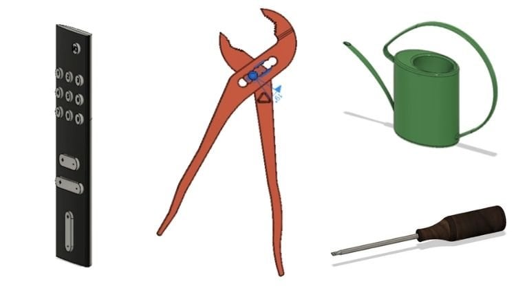So that we will deal with the design of example projects in the following. The first project, we will get right into the swing of things. Learning the design procedure based on a very simple carabiner. 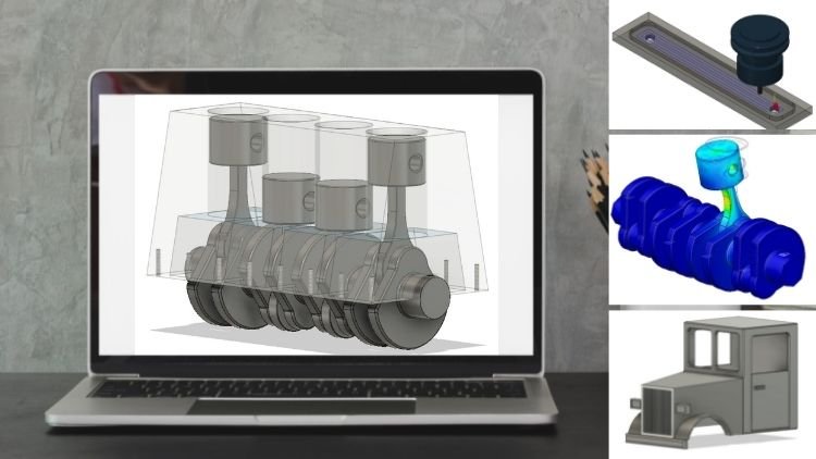This is followed by our model of an exhaust manifold, which has already a bit more difficult to implement than simplified model of attract front end. And finally, a simplified model of a four cylinder car engine where things to get a bit more complex. But don't worry, we will go step-by-step, by the way. By working practically, we will get to know even more new functions and commands, as well as consolidate the basics. So learning by doing, stay with me, it will be exciting. 10. Design Project I: Simple snap hook: For the carabiner, we start in a new single part, part with the button start to D, sketch and selection of a plane, e.g. the except plane. Let's first consider how the carabiner is constructed and how we could best design it. If we look at the carabiner a little closer, we noticed that you can put a circular shape in each of the left and right areas. The strategy of the carabiner represent the tangential connections between these circles. Let's design the Caribbean and in this way. So let's first draw the first circle with a starting point on the horizontal line, which in this case is the set axis. E.g. we choose a diameter of 50 millimeter. Then create another circle with a diameter of 20 millimeter, a little further to the right. We then dimension the distance between the two circles as 70 mm. To completely define the previous sketch, which you will see by the blue coloring, we now need a reference in the direction of the x-axis and the set access to the origin. We define the position of our sketch and set direction, e.g. by another dimension of 35-millimeter from the center of the circle to the origin. The x position simply with the dependency or constraint vertical. You can either define a sketch completely by dimensions only or choose a combination of dimensions and conditions as here. For the condition we choose the center of each of the two circles, then the origin. Now the sketch is blue and fully defined. That means it cannot longer be moved in the plane without further ado. Then we draw a horizontal and vertical guides through the centers of the two circles to make it easier to apply the dimension and tangential lines. Draw the lines and right-click on them to select the construction command. In the next step, we connect the intersection points of the vertical guides with the circles by two lines. To get a self-contained shape, we only need the outer contour, so we use the trim tool. Use the tool to remove all superfluids line segments as follows. Now, we could already extrude the surface, but then we would have to make another cut out to get the final carabiner. But we can also apply a faster solution right away and draw the cross section of the carabiner in one step. To do this, at two additional circles of 35.10 millimeter diameter in the inner area of the carabiner. And analogous to the previous steps, again, draw two lines from the intersections of the circles with the auxiliary lines. Then remove all superfluids line segments by using the trim feature again to create the cut-out for the opening of the Caribbean. At the same time, we draw a line at 100 degree from the base of the inner tangential connection line to the outer connecting line of the Caribbean. And the dimension is automatically obtained by specifying the ankle and the end points. You can switch between dimension and angle a and angle input with the Tab key. Then draw a second parallel line in dimension two millimeter distance. If the parallelism is not created automatically, pay attention to the small signs. You will have to create it yourself. With the trim function, we again remove the superfluids line segments. As you can now see, we have saved ourselves a few steps and can now extrude the finished basic shape of the carabiner right away. To turn to the surface into a 3D body. Now, we switch to 3D mode with finished sketch and use the extrude function. To do this, select only the outer surface as the profile for extrusion in the options and enter a value of ten millimeter. You can either extrude in one direction only or symmetrically or independently in two directions. You select this direction. If you want to have a conical shape, you could also specify an angle at taper angle, but we do not need that here. Finally, we are on the few edges using the Philip command from the Modify section. 20 millimeter for the back top edge, and 1 mm for the edges of the opening, as well as the sides. You can select several edges, one after the other. Flawless, before we move on to the next design project, let's save the part. If you want a different file format, e.g. for 3D printing or another program, we can create this file using Export and selecting cat format, specifying the desired file format and location. E.g. the Katia and the pro engineer formats are available as well as commonly known STL and step file formats. 11. Design project II: Exhaust manifold: Welcome back. In this chapter, we will implement the design of an exhaust manifold to increase the difficulty level a bit. In this chapter, we will work with the sweep function and for the first time, we will make a 3D sketch in addition to the 2D sketches. Before we get started, let's first consider again how to design the manifold. When we first look at it, we see that in this single part, we have two basic rectangular elements that are on two different and non-parallel planes. Between these rectangular bodies then sit the curved tubes for the ritual cylinder parts of an engine. So we can design the manifold and these three steps, Let's go. We start again in the part environment with a new single part for the rectangular element that would lead to sit on the engine. We start a sketch on the exit plane and draw a rectangle with the dimensions 100 millimeter and 400 millimeter. We select the coordinate origin as the starting point. Then we add four circles for the openings. The circle should all be the same size. We achieve this with the relationship equal and have a diameter of 60 millimeter. The distance to each other should be e.g. 90 millimeter. Now we need the dimensioning in x and inset position on this plane so that our sketch is fully defined. At the moment, the circles are movable, which is not desired. For the set position, we dimension one of the circles to the center with 45 millimeter distance. And for the X position, we use the relation horizontal, with which we link the circles horizontally with the origin. Then we finish the sketch and extrude the area of 15 millimeter. To do this, select the area between the circles and the rectangle. Then next step, we create the rectangular element that would be mounted on the center muffler or catalytic converter of the exhaust system. To do this, we need a sketch on a plane that in this case is parallel to the x-y plane. So to do this, we create the parallel plane or offset plane using the offset from plane command from the work features and plane section in 3D model. Select the command and the x, y plane and enter a distance. In our case -250 millimeter. We need the minus for the correct direction, which here is the negative set direction. On this plane, we start a new sketch and draw a rectangle with dimensions 110 millimeter and 80 millimeter. We get the fixed position in x-direction with the condition vertical between the center of the rectangle and coordinate origin. A fixed position in y direction using a dimension of 250 millimeter from the center of the circle to the origin. We also draw a circle with a diameter of 60 millimeter. Then this sketch is done and can be closed. We extrude the area between the rectangle and circle again by 15 millimeter. Great. Now we have the two rectangular geometries and then can turn to the exhaust pipes. We will use the sweep function in this chapter because we can create the geometries quickly and easily with this function. As you may remember, this function always requires profile and the path. As profile, we simply draw four congruent circles on the first created element. Now, to create the desired shape, we need to create the path, e.g. a. Line across the 3D space from the respective circle of the first rectangle to the circle of the second rectangle. This works easiest with a 3D sketch. So far, we have always drawn a 2D sketch on a plane when we created an element. But you can also sketch in 3D space. This is actually relatively easy. It just takes a little more imagination. You will also get a better idea if you just rotate the drawing plane a lot, giving you multiple perspectives. So we select the Start 3D sketch command and then we're taken to the 3D sketching area. If we select the line command, normally, we can build our path from individual lines. We start by clicking on the center of the first circle. Now we are shown a coordinate system with the three colored axes, x, y, and set. The orientation matches the coordinate system of the single-part, depending on which axis direction you now move with the mouse. You can draw a line on one of the x's. We first need to move in the y direction. That means upwards. Move your mouse upwards and sideways so that the green line, the extension of the y-axis appears. Then you can enter a dimension e.g. 80 millimeter. Now we have a line of 80 millimeter in y-direction as if we had drawn on the x y plane. Next, we draw a line of 30 millimeter in the set direction. That means the blue line must appear. To do this, we start at the center of the second element created. And lastly, we simply connect the two endpoints of these two lines in 3D space so that we get a diagonal line. With the band command, we can still round off the tooth sharp corner points with e.g. 30 millimeter. The first path for the sleep command is ready. As a profile, we simply draw a congruence circle in a new sketch on the rectangular element. When starting the command, we must first activate the profile section in the Properties window. Then we can select the first circle profile. Then we have to change the selection to path. And then we can select the first path. The program will then create our first pipe segment. In the output area, we can set join e.g. so that we joined the created bodies together. Finally, confirmed with the k. The procedure for the remaining three pipe segments is identical. The only difference is in drawing the 3D path. That means we need different length for the lines in the set direction for the element in the upper area. We had at the first path, 13 millimeter. For the second path, we need 60 millimeter for the third, 120 millimeter, and for the fourth, again, 30 millimeter dry. It. Very good. The exhaust manifold is almost done. We now need to hollow out the created solids so that we actually get pipes. We do this with the shell command. Select the command, select the lower and upper circular surfaces and enter a wall thickness of e.g. two millimeter. Great. In this lesson, we learned quite a bit the creation of a 3D sketch, an offset plane, and the practical use of the sweep and shell commands. As the penultimate design project, we will construct the front end of a truck with a passenger sell, or drivers cap. In the following chapter, this will be a bit more challenging, but together it is not a problem. We will go step-by-step again, stay with it and please continue. It gets more and more exciting. 12. Design project III: Truck front part: For the front part of the track, we start a new single part. First. Let's think about how best to build the model. We need a trapezoidal section for the hood, cuboid for the actual cap, and add on parts like fenders, headlights clearly and bumper. This means we could start with the section for the engine hood, e.g. to do this, we start a sketch on the x, y plane and draw a simple rectangle. The starting point should be at the center, and the dimensions should be 140 millimeter and width and 90 millimeter in height. Then we create the parallel plane to the x-y plane with 120 millimeter distance. On this plane, we will now sketch another rectangle which will be somewhat smaller, 75 millimeter wide and 80 millimeter high. To be more precise. The distance of the center should be five millimeter to the coordinate origin, so that the two lower edges of the rectangles are congruent. With the loft function. We can now have the two rectangles connected in 3D mode to form a solid. For the drivers cap, we then draw a new sketch with 140 millimeter wide and 170 millimeter high rectangle on the real plane of this solid. We then extrude this rectangle 120 millimeter. Now, we already have the two basic shapes for our object. For the two vendors, we draw a sketch on the y, z plane in the next step, since we want to extrude them symmetrically from the center. After starting a sketch, we first draw a three-point arc with 50 millimeter radius and 72 millimeter distance in horizontal direction to the origin. We set the two remaining points coincident. That means congruent with the left corner and once with the bottom line of the engine compartment. Then we need another three-point arc, which we said concentric to the first arc. And two horizontal lines, each 2.5 millimeter long, which connect the two corner points of the arcs. Dimension them with 2.5 millimeter each. To select a specific element, stay a little longer with your mouse at the position. Then a small dropdown menu will appear with which you can choose which congruent element you want to select. The second 2.5 millimeter dimension is no longer necessary. This results from the other dimensions and the concentric condition. This dimension would over define the sketch. So we can only use a control dimension here, which is then placed in brackets. A control dimension is not fixed, but changes when we change another dimension. So it just chose a value. In order to be able to extrude the profile in 3D mode, we must first select the profile and then the function. Otherwise, we will not be able to select the profile because it is inside. We take a dimension of 140 millimeter with symmetrical direction. If we want to create an independent body for the volume element, we select New Solid for output. Otherwise, simply join. Then it will simply be merged with the previous body. In this case, we choose join because we still want these vendors to be part of our basic body. In this chapter, we only want to create a new body for each add-on part, such as the radiator, Crilly headlights and bumper. But not the separate in the ritual part as we would do in a normal assembly. We have already briefly touched on how to deal with individual parts in an assembly and how to link them to join in an assembly in a previous chapter. We will learn about this in more detail in the next chapter. Note that in this context, buddy and component are different terms confused by buddies, parts and assemblies. Let's make a short digression about body versus single-part. The difference between body and single-part is that each assembly consists of single parts and each single part in turn consists of bodies. So it's a kind of hierarchical detailing. E.g. in a car, the parts of the chassis, the doors, the wheels, and all other parts down to the smallest bolts, are designed as individual parts. Each of these individual parts of a main assembly can in turn be divided into several bodies or even solids. But you don't necessarily have to do that. You can also build a single part from just one body, especially if it is very simple in design. In this case, we build our model as a single part, but since the single-part is somewhat more complex, we build it from several parties. This offers the advantage, e.g. that we can clearly delimit the individual bodies and e.g. hide them or slightly changed the appearance of these bodies. To summarize briefly, in conclusion, a body is, so to speak, a more detailed democratization within a single part, which in turn can belong to an assembly. Our body is primarily a component of a single part, whereas a single part can move freely within the parent assembly and is linked by joints within an assembly. Don't worry. If you don't understand it right away. You will understand it even better to ring the course based on practical implementation. Back to our truck. In the next step, we want to hollow out our solid. We do this with the command shell. I click on the lowest surface and the input of a five millimeter wall thickness. We would also like to remove the surfaces inside the wheelhouse things. On the one hand, we could start an extrusion as we know it. On the other hand, in this case, we can also simply remove the face using the delete face command from the Modify section. Please note that you have to check the option heel remaining faces. Otherwise, it will not work as desired. We will then take care of the two-part windshield. We want to build this from two simple rectangles. Take the dimensions from the following profile. Then finish the sketch and cut it out with extrusion. We'd round the edges of the windows with five millimeter. We proceed similarly for the side windows. For these, however, we draw only a rectangle on one side and then simply cut through the entire width since the cabin is hollow. Anyway. The dimensions and position of the rectangle should be as follows. To give our model also at least the appearance of a door, we will get to know a new function. The command emboss. This command. We first need a sketch, so we draw a rectangle for embossing the door on the side surface of the drivers kept. The starting point should be in the lower left corner of the window and the rectangle should be 90 millimeter high and as wide as the window. Then we select the command, emboss the sketch profile and select as effect and grief from face because we do not want an elevation but the depression and specify 1 mm as depth. As you may have recognized, this step would also have been possible with Extrude. For the door handle, we now draw a rectangle on this surface, again, this time with the following dimensions. Then we extrude the profile of five millimeter and select New Solid in operation. Because we want to create a new body for this. To make it easier for us, we simply mirror these two features to the other side. To do this, we select the mirror command and then the type options features. We now simply select the embossing and the door handle in the pot browser, and then switch to mirror plane in the options and select the y set plane as the mirror plane. Just try it one after the other in case mirroring both features at once doesn't work. The mirror or function usually creates significant time savings for symmetrical parts and features. Incidentally also in the 2D sketching environment. Therefore, try to use this function as often as possible. We continue with two fillets, one-fortieth to door handles with 1.5 millimeter each. And the two upper edges of the side windows with five millimeter each. Now we draw the bumper. This should sit at the front with the dimensions 140 millimeter and 15 millimeter. To do this, we again use the dependency colinear for the upper horizontal line that we linked to the truck front end, e.g. the left vertical line that will link to the side of the truck to fully define the sketch. Then we can extrude the profile eight millimeter. We again create a new body for it and still around off with four millimeter. For the headlights. We first draw one of the two needed on the front surface and then mirror it. E.g. the profile should have the following dimensions. We then extrude it with ten millimeter. In addition, we draw another two millimeter cut out with two millimeter distance to the headlight body to improve the design a bit. And the connecting strategy for a little more stability. For this connecting stroke, we need a circular geometry on the front side surface of the track with six millimeter diameter and the distance of 83 millimeter and horizontal to the origin. In addition, another circular geometry on the back of the headlight, also six millimeter in diameter, which we simply dimension from the top inside edges with eight millimeter, 12 millimeter. Then we use the loft command and connect to circular surfaces to form a three-dimensional connecting stroke. Now we can mirror of the headlight and the struct to the other side. As less detail of our truck front, we would like to draw a radiator grill. For this. We first start a new sketch on the front surface. Then we first draw a rectangle with 75 millimeter, with an 80 millimeter height. The sideline and the top line should each be co-linear with the lines of the front face. In the next step, we draw another rectangle with a four millimeter distance to the edge of the first rectangle, which borders our radiator cutouts. Then we draw a vertical line congruent to the center line. Then we draw a line to the left and right of the center line. And the distance of 1 mm from the center line. The start and end points should be on the second rectangle drawn. Now, we would have to draw a lot of these lines because we want to extrude every other space between them to get the shape of the cruelty. To make life easier, we will use a new command called pattern or rectangular pattern in this case. To do this, we select each of the vertical line elements. First select the left line, start the command, and then we have to specify a direction in which the pattern should be created. To do this, we simply select the upper or lower left line segment of the rectangle, and if necessary, turn the displayed green arrow with flip in the options in the desired direction, means to the left. Then we have to enter a distance of 1 mm between the line elements and increase the number 233. And wallah, the program does the work for us. We then do the same for the other side, but to the right. Now, to create the solid body of the radiator cruelly, we extrude the area between the two large rectangles and every second long, narrow rectangle two millimeter outwards to create the following solid. Excellent. After we have rounded a few more edges, according to our tastes, with two millimeter each, we take a quick look at the individual bodies and then have this less than done. Great, if you stuck with it. As we can see, we have now created several bodies and the bodies folder and the part browser, more precisely, one each for the door handles, the body, the headlights, the struts, the bumper, and the radiator cruelly. We can now hide, show these bodies as we wish or change the appearance pair body separately. If we want, we could print the model as it is with a 3D printer. If you're interested in 3D printing, feel free to take a look at my course, 3D printing one-on-one. However, if you prefer to design the bumper, they radiate to query and the headlights as independent components and then assemble them in an assembly. Take a look at the next lesson. First. The next lesson, we'll take a step-by-step look at how to work with components in an assembly will design a simplified model of a four cylinder internal combustion engine. This is going to be pretty cool. Let's get right to it. 13. Design Project IV: 4-cylinder engine (Part 1: Crankcase): As announced, we want to design a simplified model of a four-cylinder engine. In this chapter, we want to initially built this model from several main components as in reality, but will then neglect some details so that the construction does not become too complex. To start with. We need to crank case. We will omit an oil pen and the cylinder head with Ralph cover. So the first component we design is the crank case, is it creates a central starting point. Do this, we start on the exit plane with a sketch. To create this shape for the crank case as the basic body, we first spend a rectangle from the center point and can immediately specify 500 millimeter is the width and 150 millimeter as the height as dimensions. Then we finish the sketch and create a parallel plane to the exit plane in 3D mode with a distance of -250 millimeter, as we have already learned in one of the previous lessons. On this plane, we then draw a rectangle with identical width, that means 500 millimeter and the height of 250 millimeter. After closing the sketch, we use the loft command to create a trapezoidal solid. Now we take care of the host for the pistons, that means the cylinders. We can insert these in two ways, either with the whole function or as a circular cutout with Extrude. Since the holes have to go completely through the cuboid, we simply use the cutout in this case. For this, we start a sketch on the upper surface. We want to create cylinders with 90 millimeter diameter and four-cylinder engine. Therefore, we need the following dimensions and geometries. What is the easiest way to draw these circles? First, we draw a circle with a diameter of 90 millimeter and define its position in x-axis direction with a dimension of 73.75 millimeter from the center to the edge. Fully define the position of the circle. We need not only the diameter and that dimension to a fixed point in the x-direction, but also a position in the set direction. Since the center of the circle should be on the x-axis, we use a condition instead of a dimension. Select the center of the circle and the origin, and select the condition horizontally. For the second circuit, we use conditions again. First, simply draw a circle and then set the condition equal. So the circle gets the same dimension without further dimensioning. Then again, apply the condition horizontal for the set position of the circle and the dimension in X for the X position in the coordinate system. In this case, 191.25 millimeter to create an even distance of 117.5 millimeter between the cylinders. Since our geometry of the fourth circles is X is symmetric around the set axis, we can now create the two other circles very quickly and easily with the mirror command. For the command, we first have to create an axis around which we want to mirror because the set axis is not selectable. In this case, we do this by drawing a line congruent to the set X's and linking it coincident on the origin. We then convert this line into a construction or auxiliary line by right-clicking and selecting construction. You can recognize this by the dashed line type. We will not define construction lines completely since they are not necessarily relevant. We only need a defined position and x-direction which we already have. Then select the mirror command in the pattern menu and select the two circles in the options. Switched the selection to mineral line and then select the construction line you just created. With apply. The other two circles are created and are already fully defined. We close the 2D sketch and create the sections with Extrude by selecting the fourth circular areas. In the options, we can select two for distance, and then select the surface up to which the cutouts are to be made. In our case, we select the ground surface. By the way, output must be set to cut. By the way, we could have integrated these circular areas into the first sketch right away and thus saved ourselves a step. Then we mentioned the lower part of the crank case, which will later How's the crank shaft? To do this, we create a trapezoidal cut out that spans symmetric Kelly from the center of the housing. First, we draw a baseline on the y set plane and said it colinear with the crank case bottom. Then we draw the trapezoid as shown. And dimension the height, width 100 millimeter. Then dimension the lower corner points with 25 mm to the wall. For the sidelines, we choose a parallel condition to the sidelines of the cabinet. In 3D mode, we again use the extrude command and select the trapezoidal surface. Then we select the option symmetric for direction and the option cut for output. We also enter a dimension of 450 millimeter, since we have a length of 500 millimeter and want to leave 25 millimeter of wall thickness for each. Confirm and done. We now need to add material again for the crank shaft mounts. We draw the following three rectangular profiles on the lower surface of the housing. We then extrude these in 3D mode with the selection of two at distance, as well as join at operation at the extrusion options. This allows us to select the bottom face and extrude the 3 bar to it. In the next step, we create a circular cutout for the bearing surfaces of the crank shaft. To do this, we draw a circle with a diameter of 70 mm and the distance of 125 millimeter from the corner point on the sidewall of the housing. The center of the circle should be congruent with the bottom line. We then extrude this completely through the entire housing using the Cut option. Of course, we could have drawn only a semi-circle or use the trim function. Also. In the penultimate step, we would like to create the threaded holes for mounting the cylinder head and oil pen on our very primitive crank case. First, we create the holes for the cylinder head. We use the whole function in 3D mode for this. However, in order to place the host correctly, we first start a 2D sketch on the upper surface of the housing. We need ten holds for the cylinder head to create them quickly and easily. We use the pattern command from the create section. In this case, we again need a rectangular pattern. We first create the point with 20 millimeter distance from each of the lateral lines of the cylinder head support surface. Then we select the point and the pattern command. We are shown to selection fields for the directions, as well as input options for distance and number of the arrangement or pattern. If we select direction one and select the top line of the cylinder head, we will see a green arrow that should point to the right. If not, flip it with the option flip in the options of the pattern. Then we select direction to and select the left vertical line of the cylinder head. Direction should point down in this case, if not, flip it with flip. Now we can set the values for a number and distance in the options. Think of it like a table in a set direction. We need two lines, if we like, in x-direction, five rows, two times five equals ten points for the holes. The corner points should have a distance of 20 millimeter each to the edge. That means we need a distance of 150 millimeter for the pattern in x direction and 110 millimeter in set a direction. We then confirm with OK and get the desired pattern. Then we select the whole command in 3D mode and create the host by entering the specification and selecting the points. After selecting the points, we select the whole type tapped hole. Because we want to create a tapped hole. In the lowest selection fields, we can then choose which dimension the tip toe should have. E.g. we want our host beat 70 millimeter long and ten millimeter in diameter for a metric M ten thread. Also a thread pitch of 1.5. Confirm and the tip toes are created. One more hint. As already mentioned many times, there are several construction methods, sometimes faster, sometimes slower, but basically all of them lead to the goal. So if possible, think along so that you also recognize other ways for the holes, e.g. it is also possible to first create a hole in 3D mode and then use the pattern function of 3D mode and police the holes in the same way as the sketch points. Let's take a look at how to do this for the oil pan mounting holes. We select. Hello and then first the aboral surface, that means the underside of the housing. Then we determined the position of this hole and x and set direction. Simply click on the top edge first, enter a value, in this case 12.5 millimeter, and then click on the side edge and enter 12.5 millimeter as well. It is important that you do not press enter in-between, but simply select the next edge immediately. Then select the whole type as well as the specification as before. However, here we want e.g. only eight threaded holes and the dimension of 40 millimeter. Now confirm with OK, and the hole will be created. Then we select the whole and use the pattern command. The next step, we change two directions in the Options and then click on the x axis to indicate the first direction. Possibly rotate the direction of the arrow we flip and can proceed for the second direction, analogously as with the 2D sketch before. In the x-direction, we want eight holes with a distance of 67.5 millimeter between the holes. And then the set direction two holds with a distance of 225 millimeter. In total, 16 holds. In the last step for the crank case, and this lesson, we will use the filter command to round corners so that the command select the desired edges and enter a rounding radius of e.g. ten millimeter. The crank case is done. The next lesson, we'll continue with the pistons, connecting rods and piston pins. 14. Design project IV: 4-cylinder engine (Part 2: pistons & connecting rods): In this section, we are interested in the connecting rods, piston and piston pins. We start with the creation of the pistons. For this, we start with a new file because the piston is an individual single part of the assembly. We then start a sketch on the exit plane and first draw a circle with 85 millimeter diameter. Then we finish the sketch. Now, we still have to extrude the circle area. We choose e.g. 70 mm. The next step, we hollow it out and give it a wall thickness of five millimeter. Then we start a sketch on the y set plane of the piston to make a cut out for the piston pin, which later connects the piston and connecting rod. E.g. we choose a diameter of 30 millimeter and dimension the circle with 35-millimeter to the lower edge so that it is centered. We also draw the circle so that it sits in extension with that y-axis. Then we extrude the cutout in 3D mode, curating an opening. Finally, we round off the top and bottom edges with two millimeter each. We save piston rings and further detailing for reasons of complexity and time. We then move on to the connecting rod and piston pin first before mounting the pistons in the crank case. For the connecting rod, we again create a new single part, since this component is also an independent part of the assembly. We sketch the following cross-sectional profile of the connecting rod on the y set plan. We will first start with the two eyes. The upper connecting rod, I should have a diameter of 30 millimeter inside, 40 millimeter outside. The lower connecting rod I, 50 millimeter inside and 18 millimeter outside. Then we dimension the distance between the circle centers with 165 millimeter and set the two centers vertically to each other. We also set the center of the two lower circles congruent to the origin to completely define and position the previous sketch. Then we draw two vertical lines 65 millimeter long, each of which should have a horizontal distance of ten millimeter from the center of the upper connecting rod iron. We complete the profile with two tangential arcs, each of which should have a radius of 115 millimeter. Finally, we use the trim function and remove excess lines. When this is done, we can finish the sketch and extrude the connecting rod 20 millimeter, so that the transitions are not too extreme. We can round off the transition at the bottom and top with 20 millimeter in the area of the connecting rod. Also round off the edges of the two surfaces with 1 mm each. The connecting rod, in this case is also a highly simplified model. Normally, a connecting rod looks like the one in this picture. In the lower area, it is divided into two parts. The geometry is more functional and in addition, there are the so-called bearing shelves that would sit in the lower ie. Let's then draw the piston pin first before we start assembling the components. To do this, we again create a new part and draw a circle with diameter of 30 millimeter on the y set plane, which we then extrude 76 millimeter symmetrically and hollow out to a wall thickness of three millimeter. For the assembly, we create a new assembly file. The crank case is to be our base buddy. So we simply drag this into the assembly first. To do this, first, open all the parts of the engine and then click on the small window icon at the top right to display all the open windows side-by-side. Now you can click in each case in the desired window. And then in the pot Browser, drag the pod with pressed mouse button into the correct window and drop it. The crank case is then automatically aligned and fixed based on the origin. We then drag all the other parts into the assembly as well. Once we have done that, the last thing we do is copy the pistons, connecting rods and piston pins four times each. Since we have four cylinders. Then we first mount the connecting rod to the piston pin by selecting the following points as joint origins and selecting the joint type rotational. Then we assemble the package of pin and connecting rod into the piston with the help of a lateral joint origin on the pin and in the center of the pin opening on the piston. The type of joint is again rotation. Some patients is required here until the two correct joint origins are selected or found. Pay particular attention to the correct alignment of the axis at the joint origins. Now we would have to link all the other pistons, piston pins, and connecting rods in exactly the same way. To make life a little easier for us, we simply copy the already linked group of pistons, connecting rods and piston pins three more times. In the next step. To do this, we select the three components and copy them using control C, control V. We paste them into the design environment. The great thing about this is that the links are also preserved. We noticed this when we move the pasted parts, we have saved a lot of time and can delete the previously inserted parts that are no longer needed. We do this quickly and easily by selecting them and pressing the removed key on the keyboard. So much from copying and deleting parts and linked parts within an assembly. Now we have to link the pistons with the cylinders. For this, we select the join type, cylindrical and the shoulder joint origins. Now we're almost done with our very simple four-cylinder engine module. In the next lesson, we will draw the crank shaft. Let's go. 15. Design Project IV: 4-cylinder engine (Part 3: Crankshaft & Assembly): For the crank shaft, the last part of our engine, we start again a new single part. Ultimately, the crank shaft should look something like this picture. Of course, we will again proceed in a somewhat simplified way. We start a new sketch on the y set plane in the side view. Then we draw the first main bearing of the crank shaft or it's shaft journal with a simple circle, 65 millimeter diameter. The origin as starting point in 3D mode weeks through this circular surface and select the distance of 20 millimeter in one direction and confirm with OK. Since our crank shaft is to be symmetrical, we will draw only one half of it for the time being, and we'll simply mirror it later on the white set plane. We will now build up the crank shaft section by section using extrusion. You are also welcome to consider how you could construct the crank shaft using the revolve function. That means as the rotational part. And whether this is possible at all. We start for the next section of the first crank shaft cheek as a sketch on the previously created shaft journal. To do this, we create two circles, one with a diameter of 70 mm and the other with a diameter of 160 millimeter at a distance of 45 millimeter from each other, including a vertical condition between the two centers. The center of the upper circle should also be 40 millimeter vertically from the center of the shaft journal and certain line with it. That means P vertically connected. Then we draw two connecting lines and dimension them vertically with 60 millimeter length. And by means of parallel dimension with 30 millimeter to the upper circle center. The last step, we use the trim function to cut away all superfluids, lines and sections. Then we extrude this cheek 22 millimeter. In the next step, we draw the shaft journal for the connecting rod on this cheek. To do this, we draw a 50 millimeter circle that should sit concentrically to the upper curve of the crank shaft cheek. We need the dimension of 16 millimeter for the extrusion. Canvas, some way would be to draw cheek by cheek and shaft journal by shaft journal on top of each other as a 2D sketch and extrude them. Just as we have done up to this point. However, it is much easier now to use only this half. Again. The first connecting rod. This body represents more or less one-eighth of the entire crankshaft. In the following, we will now skillfully use the mirror function to save us some work. So for the second crank shaft cheek and the object and Jeff Jones sections, we simply mirror the first body. We do this by selecting the mirror command and then switching to mirror solids in the small Options window that opens. Since we only have one body, this will then be selected automatically. In the next step, we switched to a mirror plane in the Options window and select the side surface of half the Conrad's shaft as the mirror plane. We can leave join in the Options window for this step. Since we only want to get one body and the cheek is already correctly aligned. The second eighth of the crank shaft is finished. For the next part, we mirrored the previously created crank shaft part. In this step, select the body and select mirror plane. In this case, the side of the shaft journal that will rest on the crank case. Now, however, we need to change our approach a bit since we want to create a new body for the time being. So we need to select New Solid and the Options window of the mirror command. Why a new body? Because as we can now see, this quarter of the crank shaft still has to be rotated 180 degrees around. In this case, the x-axis. So that it is in opposition to the other quarter. Otherwise, all pistons would run in the same way, but only two of the four persons may always be in the same position. For this reason, we have created the new buddy because otherwise we would not be able to rotate this quarter of the shaft independently of the other quarter. To rotate, we simply use the Move buddies command from the Modify menu. Then, first select the body in the Options window in the left pane. Use the drop-down menu to switch to rotate about line. Then select the rotation axis, in our case, the x-axis, and enter an angle. We need a half rotation that is 180 degrees. Confirm with OK. We see that the shaft journals for the connecting rods are now correctly positioned. Before we continue, let's extend the shaft journal of the crank shaft, which is a bit too short due to the mirroring. Simply select Extrude and define a surface for the 2D sketch. Draw a concentric circle to the shaft journal and extrude 30 millimeter. Now we want to link the two existing parts of the now half crankshaft again to reunite the two bodies. To do this, we use the combined function from the Modify menu, select body and command in the options at output, select, join and press. Okay. This approach has now already saved as quite a bit of work. To continue at exponential speed, we doubled our half-finished crankshaft one last time. This time, we can again leave a join instead of new buddy as the connection type, since the alignment is correct. With one click, the crank shaft is finally almost done. What is still missing? Firstly, a few fillets, which we would like to do as follows. Ten millimeter on the edges of the transitions in the lower areas of the stringers. And five millimeter on the edges of the transitions in the upper areas. Incidentally, we could have integrated these fillets into the sketch of the stringers right away. And then three millimeter fluids for the edges on the side faces of the stringers and Chef Charles. In addition, we now have two ends and our crankshaft into our engine assembly and then create the joint to the crank shaft housing. To do this, we simply select the first joint origin, e.g. centered on the shaft journal we started with. And select the second joint origin centered on the main bearing of the crank shaft housing. We select Rotational as the join type. Perfect. Finally, all components for our highly simplified engine model are done. At the end of the chapter. We would of course like to link the connecting rods to the crank shaft and let our engine run. Originally. For the connecting rod and crank shaft links. We had the crank case for the time being. For better clarity, right-click on the case and select Visibility. The linkage or joint creation is again relatively unspectacular. Please, the first joint origin centrally in the lower i of the connecting rod and place the second origin centrally on the shaft journal of the crank shaft. The join type in this case is again cylindrical. Proceed in the same way for the other connecting rods. When everything is linked, we can first unhide the crank case by right-clicking on its body and selecting visibility. And at the same time make it transparent by selecting transparent. At the end of the chapter, we now want to run our engine which allele we have placed all the joints correctly. This should be no problem. To do this, we search for the joint of the crank shaft with the crank shaft housing and right-click on it. We then select Drive and have to enter a start and end point. In this case, two angles, e.g. we can enter zero decrease as the start angle and a multiple of 360 degrees as the end angle. Since we want to see several revolutions, 360 degrees is logically one whole rotation. So we enter e.g. 1080 degrees, which corresponds to three times 360 degrees. Then just press the play icon and the engine is running. By the way, with the integrated recording function. You could now record this animation. But we will see another way to do that later in Inventor studio. Respect, if you've got this far, you can really be proud of yourself. By the way, you can end the animation of the joint simply by pressing the escape key. 16. Sheet Metal: Welcome back. Let us now turn to sheet metal design in this chapter, the dedicated sheet metal section is of great importance. If you want to design a sheet metal, the commands and functions in this tab are well-designed for this. If you want to design a sheet metal buddy, you especially need 0s in dealing with Ben's taps, unwinds and other sheet metal specific elements and features. If you want to design a curved sheet metal element such as this element in practice. That means in the workshop, you need a cut piece of sheet metal and basic form, which you then bend or machine into shape. This basic shape, also unwinding, can be easily created in Inventor in this section. To do this, you simply need to construct the finished and already bent sheet and apply command. This means that you designed the desired finished sheet metal body and then simply have the program generate the unwinding. That means the dimensions and geometries for the protection documents. Let's look at this with the example shown. The procedure for the construction is now very similar, but still a bit different as if you were constructing a solid. Let's go. We start a new part as usual in the part environment. Before we start the design, we then select the convert to sheet metal button in the upper right area. The program now takes us into the field of sheet metal construction. For the base element, we then create a sheet by starting a new sketch on a plane. We then draw e.g. a. Rectangular profile in a 2D sketch for our base element, just as usual. Now, normally in 3D mode, we would use the extrude command, but we won't do that here. This is one of the biggest differences in the sheet metal construction because we are now building our sheet metal body with the two commands, phase and flange. For the basic element, first select the face command and the sketched profile. Only have to click on it. The thickness is already selected. We will see in a moment why this is so and how you can change the thickness with the button sheet metal defaults, which is located in the menu bar above at setup in the tip sheet metal. The so-called sheet metal rule can be selected and edited with a click on the pencil symbol. Here, we can also select the material. If we edit the sheet metal rule, we can set the thickness of our sheet metal and change all important sheet metal specific parameters for sheet metal constructions, like the key factor or bending properties, the bend conditions. If necessary, you can change to another material here. How do we continue now? To continue building our sheet metal body, we now use the flange command. To do this. We always select edges or sketches in the following. Since our sheet is kept relatively simple, we simply select the lateral edge of the basic element. As you can see, the program now immediately creates the material with the correct bend. In the Options window, you can change all important parameters, e.g. the bending angle or the bending position. Let's also construct the other missing elements of our example sheet. By the way, you can also use matching commands from the other sections, such as the command for creating a hole or chamfers or edge flits from the 3D model tab. In the sheet metal area. There are two important functions for beginners that we would like to take a look at. One is the unfold command and the other is create a flat pattern to further processed a sheet metal section in unbent form or to create supports for manufacturing. On the one hand, we can use the unfold command from the Modify section. To do this. First select the sheet section that should remain stationary. That means around which part of the sheet should be unfolded. E.g. this one in the Options bar, select at all bands, e.g. to select all bands, or select only any ritual bands for the actual production documents. However, it is better to use the Create flat pattern command from the flat pattern section. To do this, simply select the command and you will then be transferred to the flat pattern workspace. The sheet will be unfolded automatically. If everything fits. You can leave this workspace again with go-to folded part and then see the generated unfold in the part browser on the left. You can then export the generated development for manufacturing or create technical drawing from it. So much for the design section and the cat design. Well done so far. Be sure to continue in order to get to know or use the full potential of inventor. In the next section, we will first briefly look at Render Animation before moving on to simulation and the technical drawings. 17. Rendering and Animation: In this part of the course, we will deal with the two functions, Render Animation. These two functions can be found in the so-called Inventor's Studio. Under environments. You need it whenever you want to present already designed in new ritual parts or assemblies statically, that means in the form of photos, or dynamically that means in the form of a video for a product presentation, for a website, for a meeting, or simply for your circle of friends. It is, so-to-speak and integrated photo and film studio for the constructed objects. In this lesson, we will first start with the render function. We will use as an object one of our construction projects, namely the exhaust manifold. As you can see, the program environment has hardly changed. On the left is the pop browser, and at the top is the Render tab with the individual functions or commands. By the way, rendering here simply means that the graphic or image is generated from the geometric information of the cat pot. You could of course, just take a screenshot if you're in a hurry. However, rendered graphic will be significantly different in resolution and realism. We'll also take more time to create. Let's just try it out step-by-step. First, of course, you can hide all the elements you don't want in the browser by right-clicking on an object and selecting visibility. But this is not necessary in our case because we only have the exhaust manifold as a single part. In the second step, we can change the appearance of our object. We can use this to apply the appearance and texture of certain materials to our entire design object or just two individual surfaces. However, this function is independent of the render tab. We have to switch to the familiar tools tab. For this. E.g. we could simply have the exhaust manifold displayed in copper. Wants to do this, first, select the interatrial part with the mouse, press the appearance button, then search for the material in the material library and added to the document by clicking on the small arrow in the right-hand area. Perfect. By the way, the final result is only shown when everything is rendered. In the scene area. We will then find a few commands with which we can edit our stage set, so to speak. That means the background and the environment. Here, you can select the preset setting with studio lighting styles, e.g. warm light, with a right-click and activate, it will be applied. Local lights can also be used to place spots for more light at specific locations. To do this, simply select position and target and the spot that better eliminates this location will be placed. The same procedure can be used to place a camera, which can then be selected during the rendering process. It is best to try out many different settings so that you find something that suits you best on an individual basis. The actual rendering is now started with the Render Image command. Simply click on the teapot icon and then make the desired settings. Here, you can set the desired size of the rendering and select either the currently displayed view or perspective on their camera, or as mentioned above, a graded camera. The lighting style can also be changed again. In the menu item. Output directory can be set so that the image is saved immediately after rendering. And then the menu tap renderer settings can be made for the duration of the rendering. But you can also leave the default values. The higher the resolution and render quality, the longer it will take. Then just thought the rendering and weight the file and the progress will then be displayed. With a click on Save random image on the top right. You can then save the random graphic. That's it for rendering. There is not much more to talk about in this environment. We will continue with the animation environment and then move on to more exciting topics. For the animation function, which can also be found in Inventor's Studio. We use the constructed model of our four-cylinder engine with a click on the button animation timeline. We first showed the timeline that opens in the lower area. We would now like to create the kind of video in which the pistons move up and down and the cylinders, unfortunately, the existing joint of the crank shaft cannot be animated in this environment. Because joins are not displayed in animation. Constraints, on the other hand, are displayed to us and can also be animated. I had already mentioned this at the beginning. Therefore, if you are planning to animate, it makes sense to use constraints in the design or at least apply them specifically for animation. This is what we will do in the following. The animation is then very simple. To do this, we need to replace the choice of the crank shaft with two constraints. We close Inventor's Studio for the time being and search for the joint of the crank shaft in the assembly environment. Since we want to replace this joint, we suppress it by right-clicking and selecting suppress. Alternatively, you could also delete it, but then it is permanently gone. Then we can move the crank shaft freely again. Now we have to reconnect the crank shaft to the crank case with constraints. For this, we first use the constraint insert to link the axis of the crank shaft and the susceptibles and the housing. Then click on the left edge of the middle phase of the crank shaft mount and select the counterpart in the housing. In the options, we have to correct the alignment. To do this, we select aligned for solution and an offset of minus five millimeter. The crank shaft is then correctly centered. The crank shaft is now rotatable, the mounted in the crank shaft housing. To get a complete definition, we still create an angle dependency with the constraint angle. We also need this for the animation. For this, we link the exit plane of the crank shaft with the X, Y plane of the crank shaft housing. For solution, we select directed angle and enter an angle of 90 degrees so that the pistons align as shown. Perfect. Now we have defined the crank shaft with constraints instead of a joint and can switch back to the Inventor's Studio area. One more tip for very simple and quick animations. You can also simply do without the animation in Inventor's Studio. Instead, animate the crank shaft joint in the design environment as we had already done and create a screencast video, that means a screen recording. Before we start, we have to set the cursor in the timeline to a duration, e.g. to 10 s, because that's how long our animation should last. In the following, we would like to animate a few revolutions of the engine in these 10 s, as well as make the crank shaft housing transparent in the course. For the first part, the movement, we select the constraints command in the animate area and then the angle relationship from the browser at the crank shaft. We must now determine the positions for start and end. The start position is 90 degrees. We leave it like this. As n position. We select e.g. 1170 degrees. Why this number? Because we want e.g. three whole revolutions. One complete revolution has 360 degrees. Three times 360 degrees for the three revolutions gives 1080 degrees. Then we have to add our starting point, which is 90 degrees, and we get the 1170 degrees. The start and end time is already entered because we have set the timeline to 10 s for the second part of the animation, that means to make the crankshaft housing transparent, we select the fade command as a component. We choose the crank shaft housing and will lead to transparency. Start with 100%. That means no transparency and increase to e.g. 50 per cent until the end of the process. E.g. we want this process to start at the first, second and to finish at 3 s. That means two Last 2 s. To do this, we select specify for time and enter the values for start and end. Finally, confirm with OK. At the end of the animation, we could reverse the transparency. Again. We do this in exactly the opposite way with the same command. First set the start time, e.g. to 7 s and the N time to 9 s. Then the program automatically adopts the value 50 per cent. For the start of the transparency, we enter 100 per cent as the n value. Where are we good? With a click on play in the timeline, we can let the animation play. Cursor must be at the beginning. By the way, with the button expand Action Editor on the upper right side of the timeline, we can view all created animation commands and edit them again. With a click on Render Animation or on the small red button in the animation timeline. We have to render our animation with the desired settings to a video and can then save it. Superbly done. That's it for the animation and rendering section. And the Inventor's Studio. We will continue with a very exciting area of inventory. In the following, we will deal with FEM simulations in the area of stress analysis. Be sure to continue. 18. Introduction to FEM simulation and simulation of a single part: In this last part of the course, things get really interesting because we deal with the environment, stress analysis and the creation of technical drawings. With the section stress analysis, you can simulate loads and material behavior. Possibly the term FEM, that means the finite element method, already means something to you. Without going into detail about this complex mathematical principle, you should at least have heard the name once and know that FEM software can be used to simulate loads and material behavior of a component. In this practical course, we will deal exclusively with the application of the methodology. After that, we will take a look at the creation of technical drawings. You need these for the transmission of information to the machine production and for documentation purposes. We would like to use the carabiner created in one of the design projects as a sample to get acquainted with the stress analysis environment of inventor. In this environment, we can simulate loads and get as a result, e.g. the resulting stresses in the component or the resulting displacements. So in simple terms, e.g. the bending of a component under an applied load. First, we have to create a load study. With create study, a window opens in which we can select which simulation we want to run. In this beginner's course, we will deal exclusively with probably the most common application, static loading. Therefore, we select this one. We can leave the set values as they are. This load study is then displayed to us with all relevant options and settings on the left and the part browser. In the analysis section in the upper menu bar, there are all the settings we need for the simulation. If you want to have different load situations calculated, e.g. simulate two different force application points. We can also create several studies. To do this, we would simply click on Create study again. For the simulation of a load on a component. We now proceed successively in four steps. This procedure is relatively identical for each study. Only the content differs. The first step is to check if the correct material is assigned for our part. To do this, we use the materials menu with the assigned command. Clicking on Assign opens a window that shows us the respective materials for all components. In this case, we have only one because it is a single pod, depending on what we selected as the material during the design process. The material is displayed to us under original material. In the override material field. We can now select the material of the part for this study. Currently, it is set to S defined, so the actual material of the object will be used for our load study. If you want to select the different material for, say, different loadings, then we simply select it from the drop-down menu. Alternatively, we can change the material in the design environment, but this will be more laborers for multiple studies. For the simple carabiner, e.g. we now select aluminum for the calculation wants, since deal would have much too high Young's modulus for opening the carabiner here. That means it would provide to high resistance to deformation. For the calculation of the safety factor, the yield strength of the material should be used. That means the point in time from which plastic deformation occurs in the material due to the load. However, if necessary, we could also select the ultimate tensile strength. That means the maximum stress that the material can withstand. The second step before we can start the calculation of the simulation is to select constraints and contacts. For the calculations. We only need contacts for an assembly with several components. Because with contacts, we define the load transfer when the individual components, that means the connection points between the components. However, we will take a closer look at this in the second example. Here, we only have to define constraints. Constraints simply represent constraints in the simulation area. That is, at which points are surfaces are, component is fixed in space or how, or where it is supported. Imagine it in a very practical way. You would take the carabiner in one hand and hold it with the palm of your hand against the back, or press the back against the palm of your hand. So we select the back surface of the carabiner as the bearing. For this, recreate a constraint with the command fixed from the menu section constraints. Here, we can choose between fixed pin and frictionless. For the carabiner, we select fixed as the simplest constraint and assume as a simplification that this applies in all directions. That means that the carabiner does not move a bit in the palm of the hand. Then in the third step, we still need a load. Of course, we consider how the carabiner is actually loaded. In the present geometry, the front element of the carabiner is loaded by pressing it so as to widen the opening of the carabiner in order to thread a rope, e.g. e.g. one will press with the index or middle finger against the upper edge of the carabiner. That means just before the opening. For the simulation of this load, we select the command loads and S type of force. We could also apply a pressure load, a moment or other load here, depending on the situation. Then we select the front upper rounding of the carabiner just before the opening and enter a value for the force of 100 Newton e.g. this corresponds to a load of approximately ten kilogram. Incidentally, a man can apply up to 500 Newton of gripping force as standard. That means approximately 50 kilogram. If he exerts himself more strongly, we assume perpendicular direction of force on the surface here. However, we could also change the direction of the force vector in the fourth and last step. Before we can start the calculation and get the results displayed, we have to generate a mesh. In the FEM method, the calculation is performed using a mesh with nodes which is placed over the solid body. We do this by simply clicking on mesh view in the upper menu bar on the mesh. The generated mesh will then be displayed. In fact, you could also skip this step because the software automatically creates the mesh during a calculation. Anyway. Afterwards, we let ourselves calculate the results by pressing the simulate button at the top and starting the simulation will run. After the calculation. The results are then displayed graphically using a color gradient. The color gradient in the component indicates which value is present, in which area. At the moment the font Mesos stress is selected in the pod browser. That means the equivalent stress according to the shape change hypothesis. In the area of the lower curvature of the component, it can be seen that a stress of probably about 180 megapascal freeways. To display the displacements or the safety factor, we switched to the respective result in the area of the part browser. When displaying the displacement, we see that we could open the cabinet by approximately 1.8 millimeter in the negative x-direction with the applied force. On the one hand, this is graphically exaggerated here, but on the other end, it is of course, too little to open the cabinet. We will therefore have to apply more force and if necessary, reinforce our carbonyl in the lower area if the safety factor we're no longer sufficient. Perfect. That was the first part of the simulation section. With this knowledge, we can already simulate a simple component to a load situation. In the second part, we will take another look at our engine model. Stay tuned. It continues in an exciting way. 19. FEM simulation of an assembly: In this chapter, we want to deepen our knowledge and skills in simulation by means of an assembly. Here, there are a few small differences to individual parts to consider. We will choose our four-cylinder engine as a model. For this, we start a new study in the model of the engine. Before we begin, we will first simplify the model for our purposes. We want to simulate the forces acting on a piston. And for this, we will only consider one piston with one piston pin connecting rod and the crank shaft. Therefore, we remove all other components. You can do this easily by right-clicking on the unneeded components in the pot browser and selecting Exclude from study. For a better view, we additionally suppress the reusability of these components. The simulation in an assembly runs a relatively identically to the simulation in an individual part, means we must first select the correct material. In our case, we choose steel for all components. In the next step, we need to define the constraints and contexts, what constraints are, and how we define them. We had already covered in the previous chapter. In this chapter, however, we also need contacts because we need to determine how the load that relate to or want to apply vertically from above. The piston surface is transferred via the components. Contexts therefore defines the load transfer between the individual components. That means the connection points between the components. There are two possibilities here. We can let the software to create automatic contacts or use manual contexts. That means create all contexts ourselves. In general, it has proven to use automatic contacts first and then to check them manually, if necessary, to modify them according to one's own wishes. If we have activated their command automatic at contexts, we see the created contexts in the browser, in the folder contacts. In our case, we need contacts between piston and piston pin, between piston and connecting rod, and between connecting rod and crank shaft. With the right-click on a contact and edit. We can edit it. We can then select the contact type as type. We have six basic contexts types available. Automatic contacts has the type bonded selected by default, which corresponds to a fixed or bonded connection state. In our case, we will leave all contacts types set two bonded to perform a simplified calculation on our anyway, simplify the model. However, we will briefly look a bit more closely at how we would select the correct contact type in a manual contact creation. To do this, it is important to know the individual contact types. The most important ones are bonded, separation and sliding. There are also shrink fit and spring and combinations with and without sliding or separation. Bonded, as mentioned earlier, gives a fixed connection glued together, so to speak. Separation allows bodies to move away from each other during loading. Sliding does not allow components to move away from each other. The surfaces can move tangentially to or from each other. That means slide on each other. However, in our model, as mentioned, we only use automatic contacts in this beginner's course. What are we still missing for calculation? Exactly constraints. That means the fixation in space as well as a load that is applied. As constraints, we select all crank shaft surfaces with which the crank shaft is mounted in the crank case. We fixed them in all directions and select as type fixed. That means we simulate in this case that the crank shaft does not move normally, it would rotate. However, we only want to simulate static and not a dynamic case. Finally, we define a load perpendicular to the piston surface, e.g. 1,000 newton. Now, we could generate the mesh, but with a click on simulate, the software will do it for us automatically. After the model has been successfully calculated. We can again display the desired results, such as stress, strain or the safety factor. In our case, we can see how the connecting rod would deform under the load. Of course, this is again very exaggerated here. Very good. That should be enough for us as an introduction to the world of FEM simulation with Inventor, you have learned how to perform a load study on a single part and on an assembly. More advanced case studies and other applications would go beyond the scope of this beginners course. Look forward to a continuation in the advanced course in Venter, like any other professional cat program, also offers us the possibility of creating technical drawings. We can then pass on to a manufacturing company. We will see how this works in the next and last chapter. Now we're almost done. Let's move on to the last chapter. 20. Create technical drawings with Inventor & Credits: Welcome back to the last chapter of this course. As already mentioned in the previous chapter, we can of course, use in Venter to create a technical drawing for a manufacturing company. For this, we will create a very simple single part which would be manufactured e.g. by CNC machining. Please designed a very simple example part on your own using the following dimensions. Then we add 45 millimeter holds to our simple model, which should go through the component and have a distance of five millimeter to the upper and lower edge and 15 millimeter to each of the side edges. To create a technical drawing from this cat model, we create drawing with file and new. First, we decide on the paper size or template. The program then takes us to the technical drawing environment. In the first step, we have to place the base view of the component on the drawing. To do this, we select the base command and then the component or its location. We can also make many other settings here, but we don't need them except for scaling for now. After we have scaled the drawing view a little larger, we create the first view width, okay. A technical drawing is created in the form of a three panel view, depending on the so-called folding. In simple terms, this means that the component is shown from above, from the side and if necessary, from the front in order to be able to place all the necessary dimensions and other designations. In addition, an isometric view is usually added to facilitate spatial imagination to place a new view, in this case, a derived view on the sheet. We use the projected command and create a desired second view by clicking on the component from which we want to derive a view. Depending on where we move our mouse cursor. The reference view is derived, e.g. if we move up or down, the view from the front or back of the component is displayed. And the same applies to the sides. If we move diagonally, we are shown an isometric view. To place one or more views, we click on the drawing layer. When we have placed all the views we want, we create them by right-clicking and selecting Create. The isometric view seems a bit too big. So we edited with a right-click and edit. In the top-left menu. We could also create a section view, a detail view, and the Breakout view and more. The main dimension function and various annotations are located in the annotate menu section. With the help of dimension, we can create dimensions for our component. This is almost the same as creating a 2D sketch, except that in this case, we provide our finished part with dimensions that are already defined and serve as information for manufacturing only. With the elements in the Symbols area can also draw geometric information, such as a center line or in this case, symmetry lines and circles centers. For the symmetry line, we simply select two parallel lines of the component. And for the circle centers, we simply select the desired holds or circles. By the way, with a click on the dimension designations, we can also edit them or add further data such as a number. Perfect. Now, all the information that a company needs for manufacturing would already be on the drawing. All lengths and widths, as well as the positions of the holds and recessive are dimensions. If special characters are needed to indicate shape and position tolerances, surface finishes, or even other texts. They can also be found in the Symbols area. The easiest way to create another sheet is to right-click and select new sheet. If we do not have enough space on one page. After the title block has been filled with designation, drawing number, material, and other information, the drawing can be saved and printed with export, e.g. as an PDF. Great, you did it with this chapter. We finished the beginner course for inventory from Autodesk. Now it is your turn to deepen, or do you have learned and above all, to apply it? You should now know the most important functions of inventor. And you can tackle new projects, cat designs, simulations, and everything that goes with it on your own responsibility. Congratulations. You've learned all relevant operations and features for beginners in this course. This allows you to design, simulate, render, animate, and fabricate your own cat files in a quick and easy way. Together, we have accomplished quite a bit in this course. Be proud of yourself if you have made it to this lesson. And as mentioned at the beginning of the course, take a look at 3D printing as well. It's tremendous fun and has great benefits when you can materialize your own designs. This way, you can create parts out of air and have a solution at hand for all kinds of unavailable but urgently needed spare parts or anything else. The best way to do this is to use my course, 3D printing one-on-one. If you like the inventor course, I will be very happy if you leave me a rating and the short feedback, as well as recommend the course. Thank you very much for that. See you soon.