3D Trees with Blender Geometry Nodes

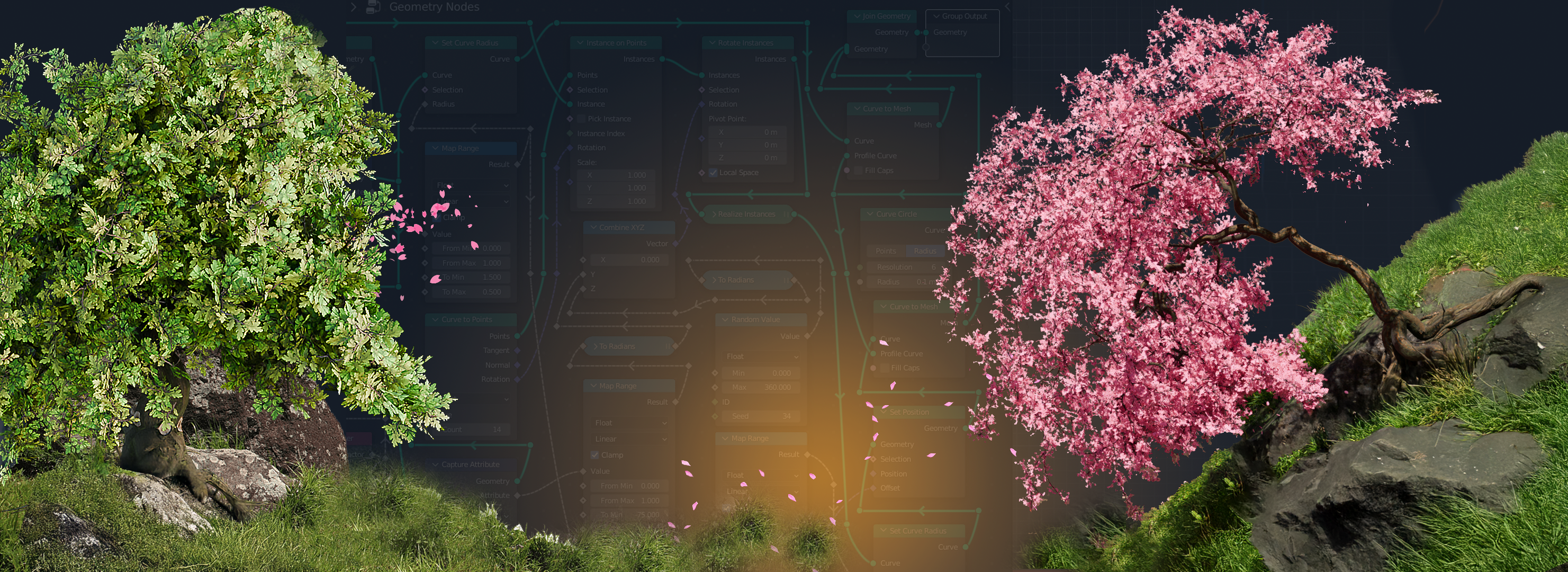
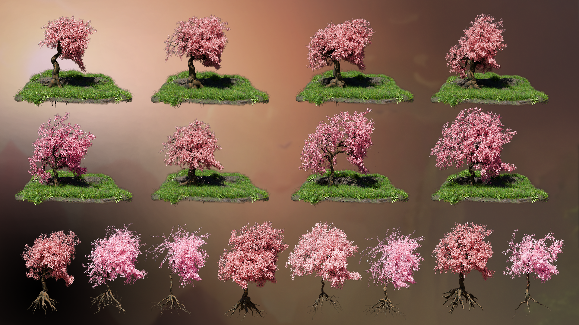
1. 3D Trees with Geometry Nodes Course Introduction: Welcome to three D trees with Blender geometry nodes. In this course, we will explore the powerful procedural workflow of blended geometry nodes to create fully customizable and realistic trees. From generating organic trunk structures to finally distributing leaves, you will learn how to craft natural looking trees with procedural flexibility. 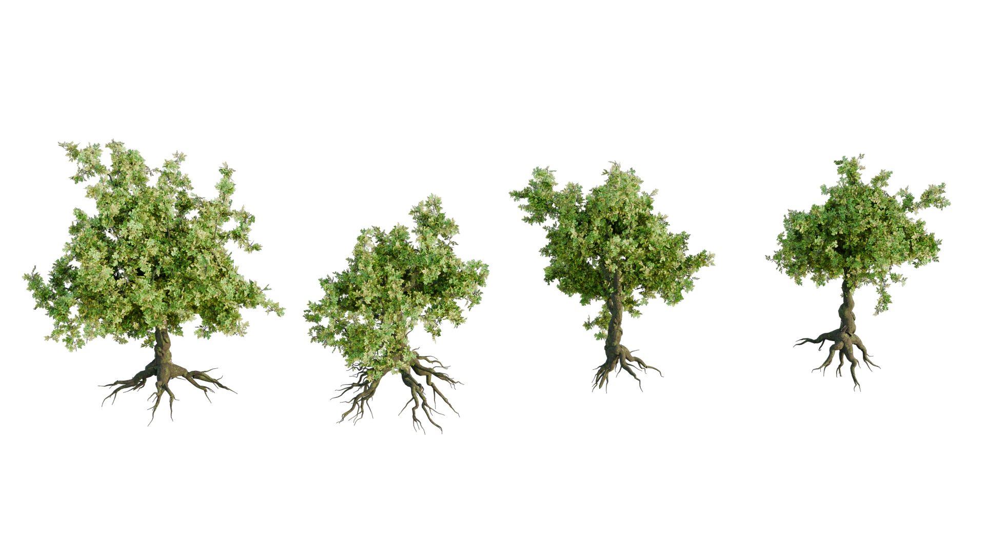By the end of this course, you will have the skills to create trees ranging from ancient oaks to delicate bonsai, all controlled by easy to use perimeters. If you are interested in pushing your gemenude skills even further, don't miss our blender geometernode for beginners, procedural bridge generator, and foliage scatter courses. 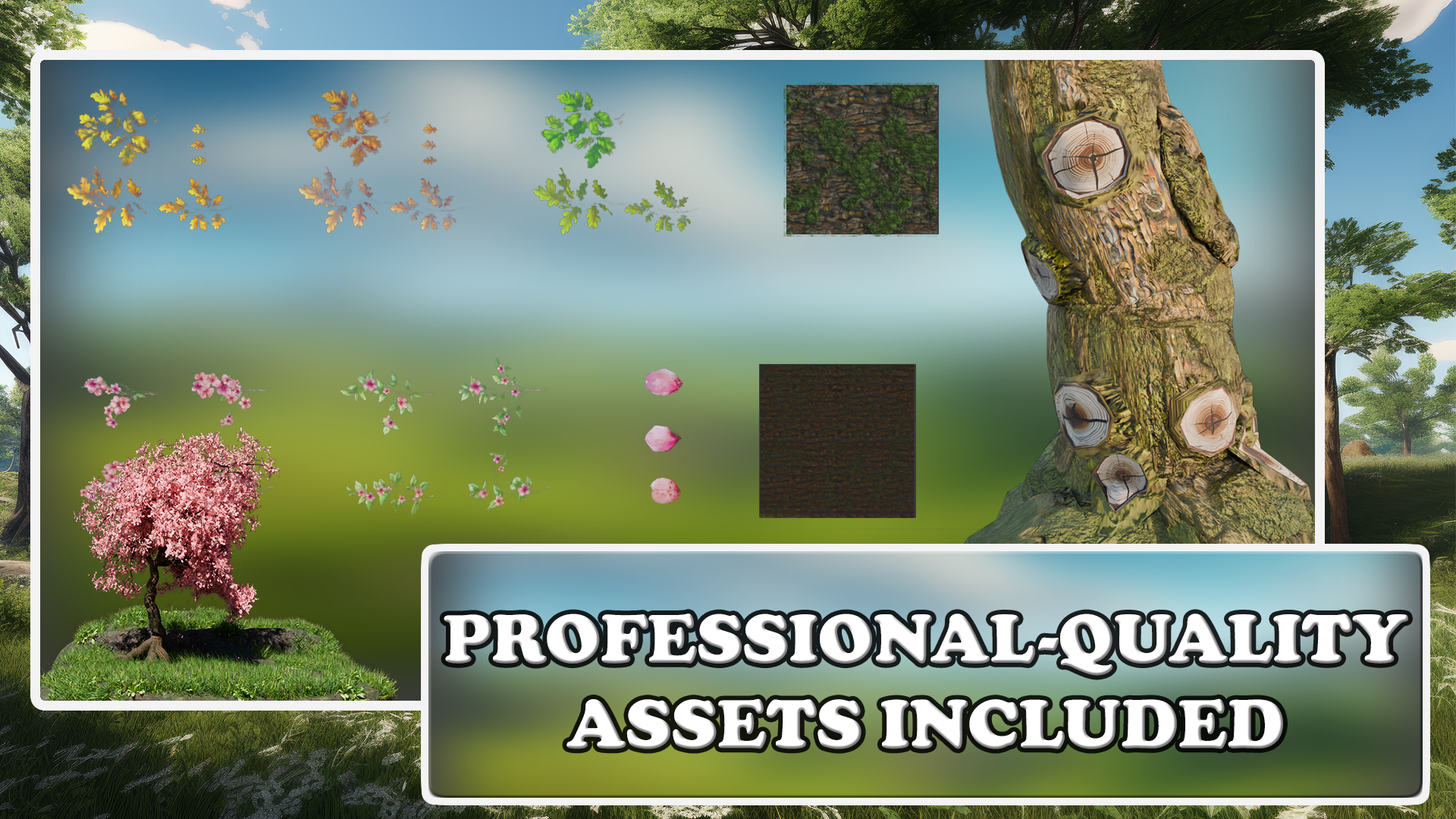These will help you refine your procedural modeling techniques and create stunning freedy environments filled with foliage, architecture, and more. 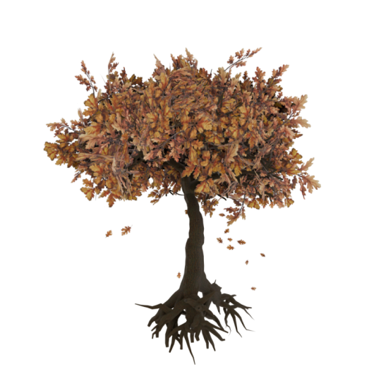To help you bring your trees to life, this course includes a high quality resource pack, featuring eight stylized PBR materials crafted specifically for procedural recreation. You'll get cherry and oak bark, blossomed and non blossom cherry branches, and seasonal oak leaves for summer, autumn, and spring, plus cherry petals for stunning falling leaf effect. We will begin by building a procedural tree system from the ground up. You will start with the foundational split end node, a custom node group that generates branching structures by iterating multiple curve splits. Using perimeters like branch count, length, and angle, we will craft a realistic growth system that mimics natural tree formation. Additionally, we'll implement a noise displacement to introduce subtle movement and realism to the tree's overall form. Once the trunk and branches are in place, we will shift our focus to leaf placement. Using custom attributes such as lengths from start and lengths from end, we will determine how leaves are distributed along the branches, ensuring natural growth patterns. Next, we'll extend our procedural system to generate roots. By modifying the branch system to reverse its direction, we'll create an underground root structure that connects seamlessly with the trunk. Finally, we'll explore UV mapping techniques, ensuring that bark and foliage materials are applied seamlessly. In the final section, we will integrate a simple particle system to simulate falling leaves. Using blenders simulation zone, we will generate and animate leaves that detach from branches over time. This course is designed with modularity and efficiency in mind. By using reusable node groups, you will be able to quickly adjust perimeters like tree height, branch density, leaf coverage, and more. Whether you need a stylized tree for game or hyper realistic op for an animation, our setup will allow for rapid iteration and customization. By the end of this course, you will have a fully procedural tree system that's customizable, efficient, and visually stunning to bring your creative vision to life. Join now and start growing your own credi trees with Blenders omiton rods. 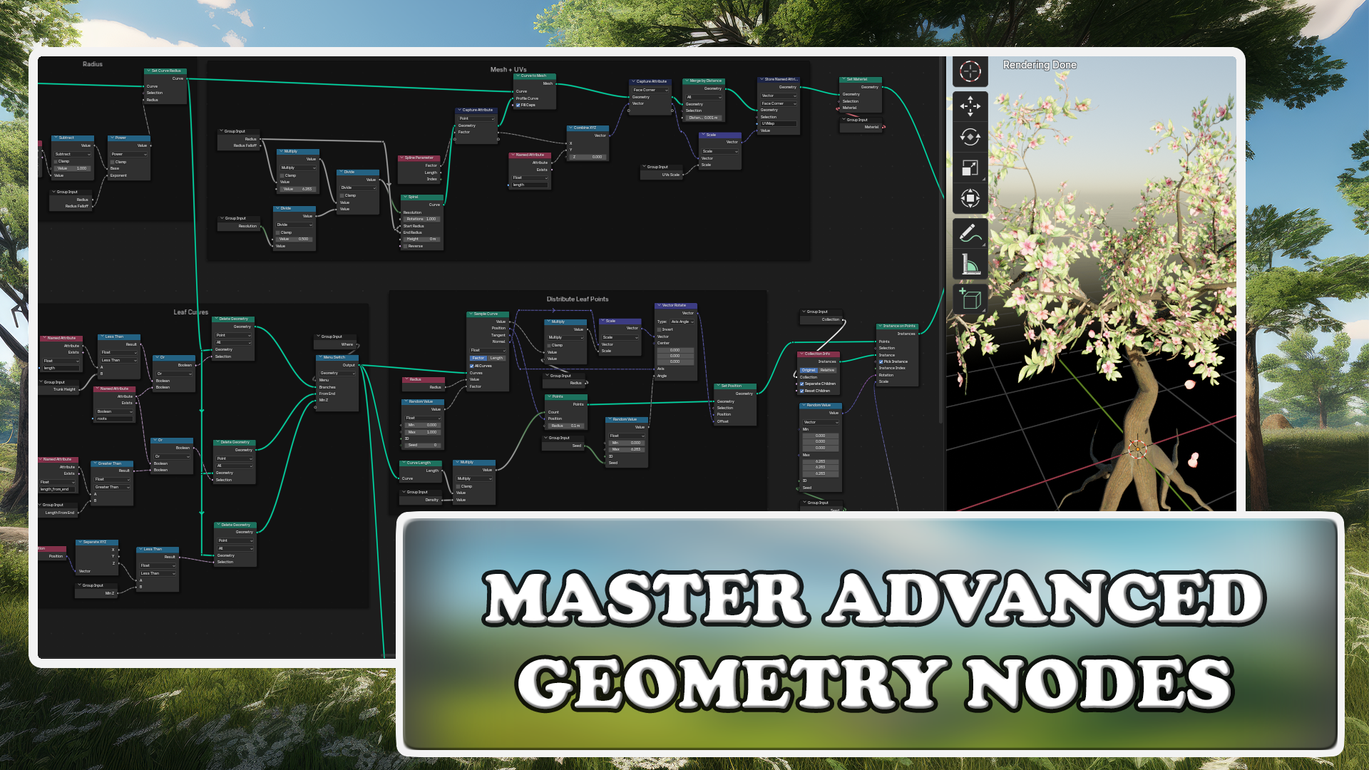2. Tree Generator Overview: Hello, and welcome to the introduction to free D trees with blender geometry nodes. In this course, you will learn how to create a fully procedural tree using blenders geometry nodes. You will build a realistic trunk and branching system, control leaf placement, and add a simple particle system for falling leaves to bring natural movement to your tree. To help you along the way, you will also receive a free material pack with high quality oak and sakura textures and materials perfect for this course and future projects. Before we start building, let's go over the inputs and perimeters that will control your tree shape and structure. 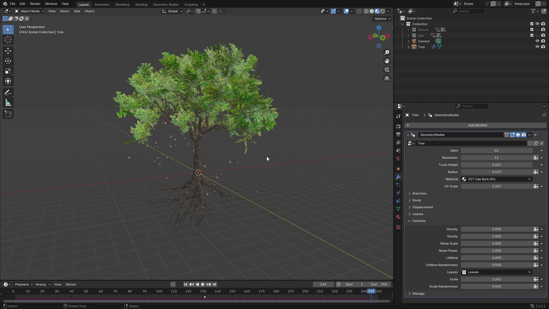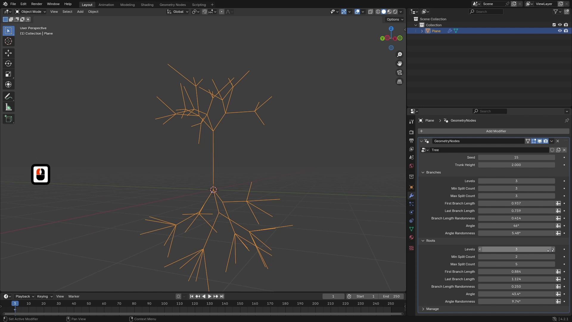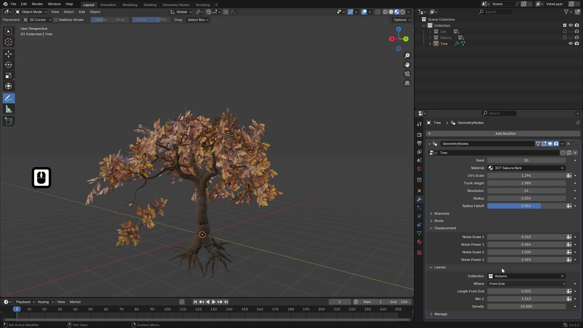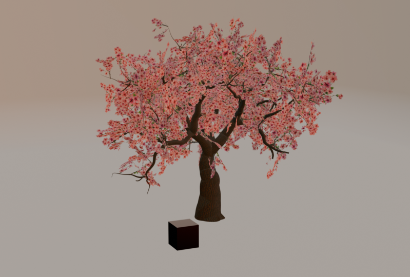By tweaking these settings, you'll be able to create anything from small bone site to massive oak. So this ometer node is just a one modifier. So as you can see, I have here this tree modifier applied to this object, and you can see that right here, we have few parameters. One of them is seed which controls seed of all of the random values and random generators. Then there is resolution which controls resolution of branches. You can set height of the trunk and overall radius. And then there's also material for roots and branches and also controls for the UEs. Then in branches panel, you can see that first input is called levels, and that controls how many levels of branches your tree will have. So if we set this to just two, for example, so first, there is a trunk, which is a separate branch or one main branch. From this branch, there are three more branches like this. And from these branches is the second level of branches, so it looks something like this. The second two inputs are min and max split count, which means you can control to how many branches each end of the branch will split. So here we have 3-5. If we set it 2-5, you can see that now it just splits to two branches. And if we play around with seed, we should get some different results. Now you can see we have four of them and so on. Then you can also control lengths of branches. You can control first and last separately. So if we set first branches to something long and last to something short, you'll have different results. And there's also a length randomness, which controls how randomized the lengths of the branches are. The next thing is angle, which controls the angle of branches. So you can see if we set it to zero, they are all pointing upwards, and as we increase it, the tree gets much wider and the branches are growing more to the side. You can also control the randomness of this angle, and the last input is radius fff, which basically controls the thickness of the branches. So now you can see it's set to two, and you can see that the branches at the ends are thin. And if we decrease it, you can see that they get much thicker and you can control the gradient of the radius going from the trunk to ends of the branches. 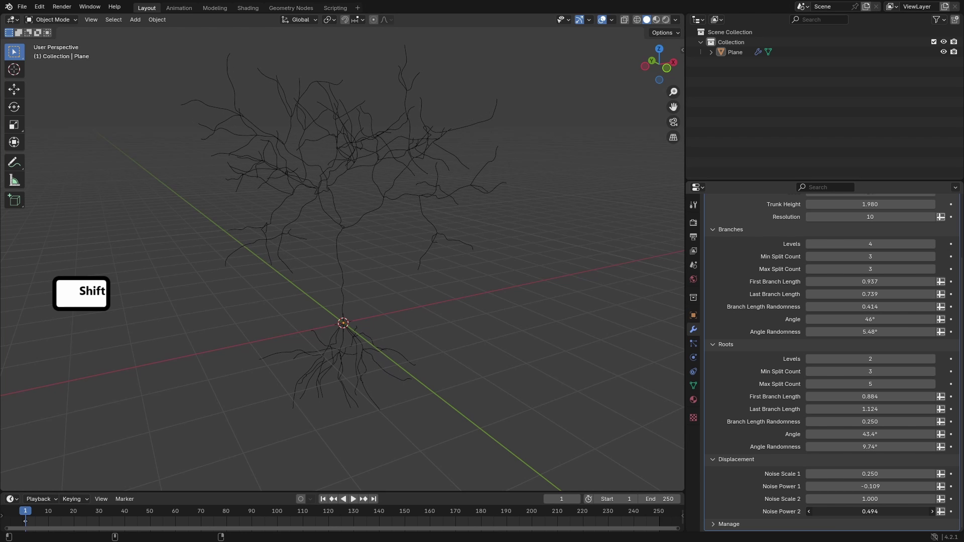The next panel we have are the roots, and this panel has basically all of the controls as branches, and you can control same parameters. So I will skip this one. The next one is displacement with which you control the displacement of the branches. 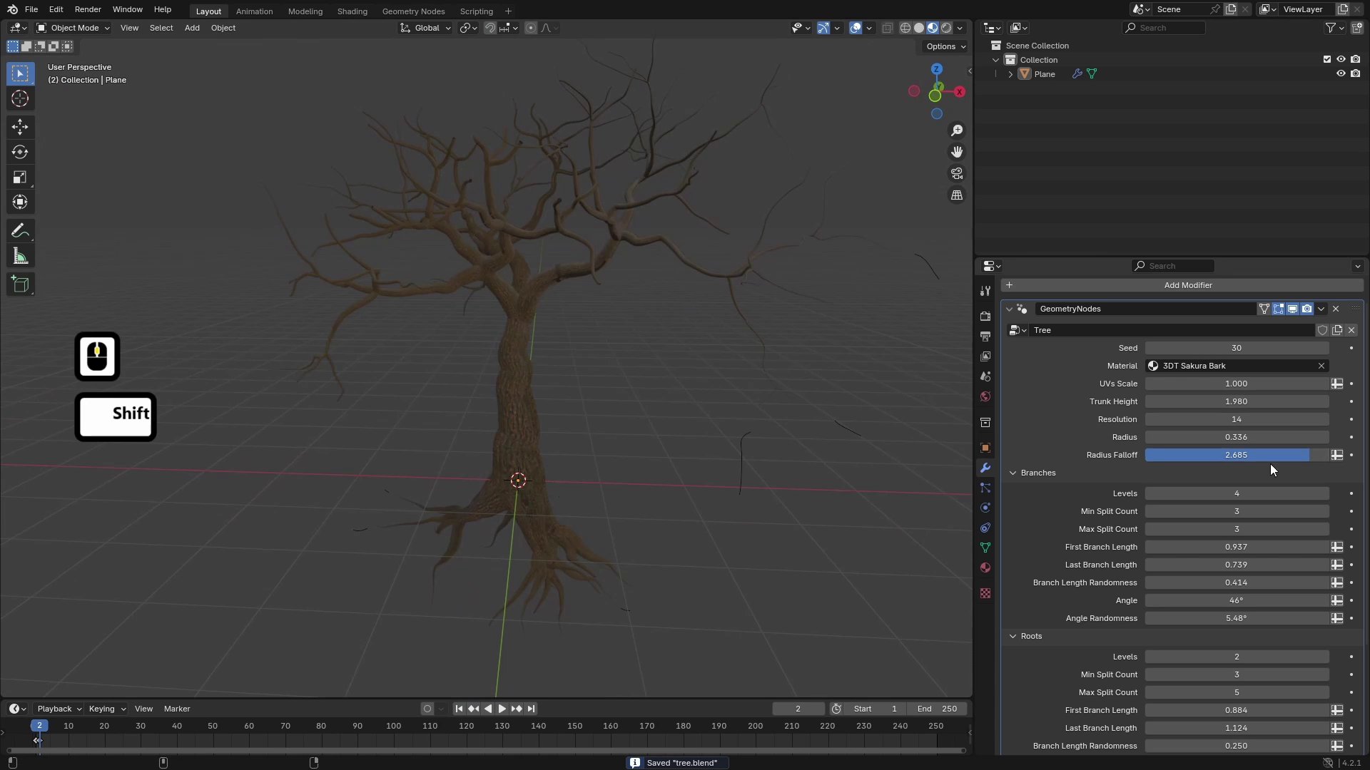So you can control how straight or how quigly your tree is. The next one are trees. So here, we can control the trees. You can select collection of the leaves. So we can easily swap between those. We can also control density, and we can pick from three options where we want the leaves to grow. So there are three options. One is branches. That means that leaves are all over the branches. The second one is from end, which basically distributes the leaves only at the ends of the branches, and we can also control the length of the segments on which they are distributed. And the last option is minimal Z position, which basically distributes leaves everywhere where the position is higher than some value. So if we said this to three, you can see that here we have level three and where the position is greater, the leaves are distributed. 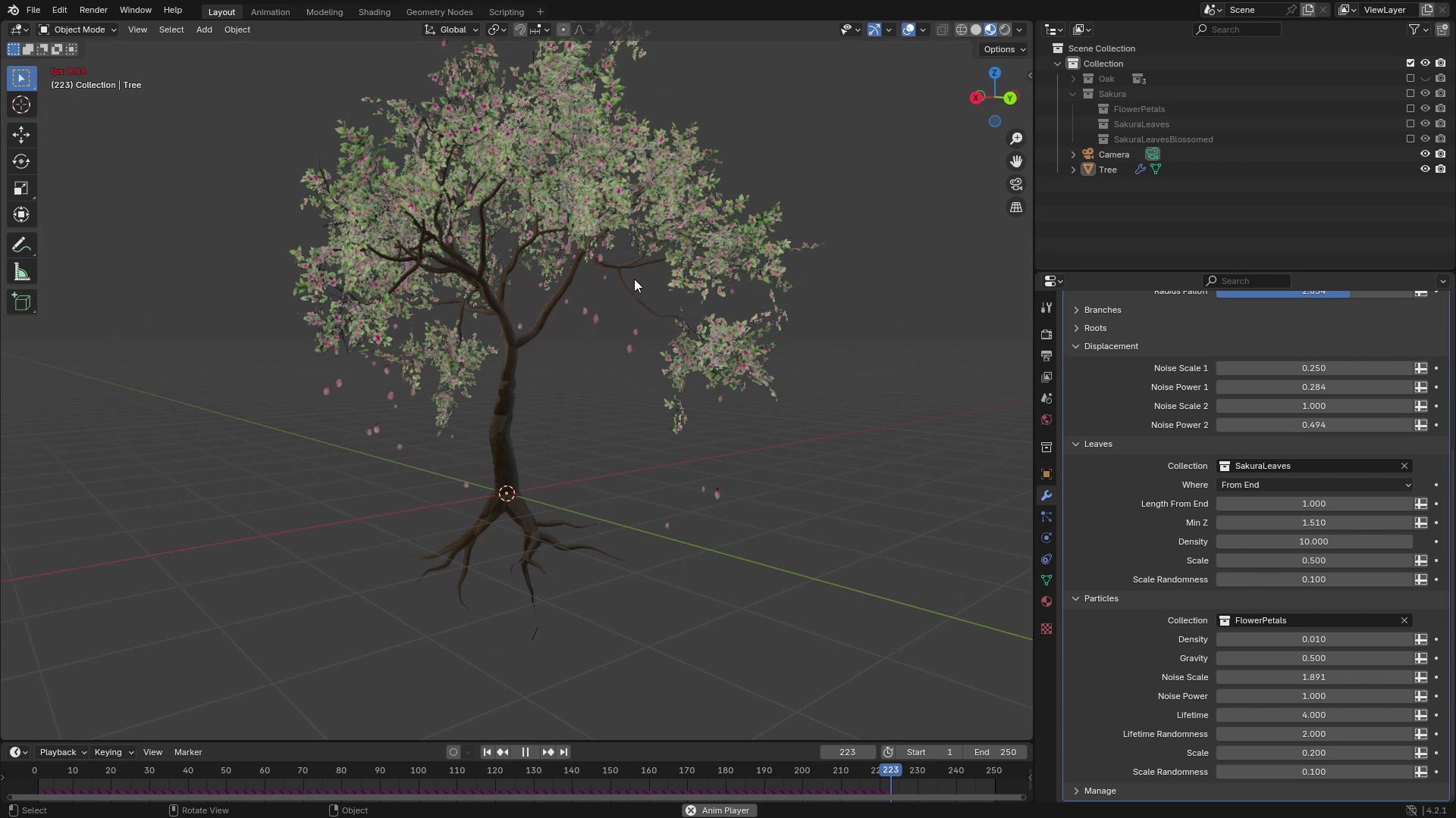The last two things are scale and scale randomness, so you can also control how scaled the original objects are. And the last panel which we have here are particles, and you can see it here. Those are the small leaves which you can see, and you can control their density, also physics, so we can control the gravity and some noise which is applied to their movement, and also how long they live. And same as for the leaves, we have collection for input objects and their scale. You can see that if we play the simulation, you can see that the leaves start falling from the leaves, and it creates a really nice effect. 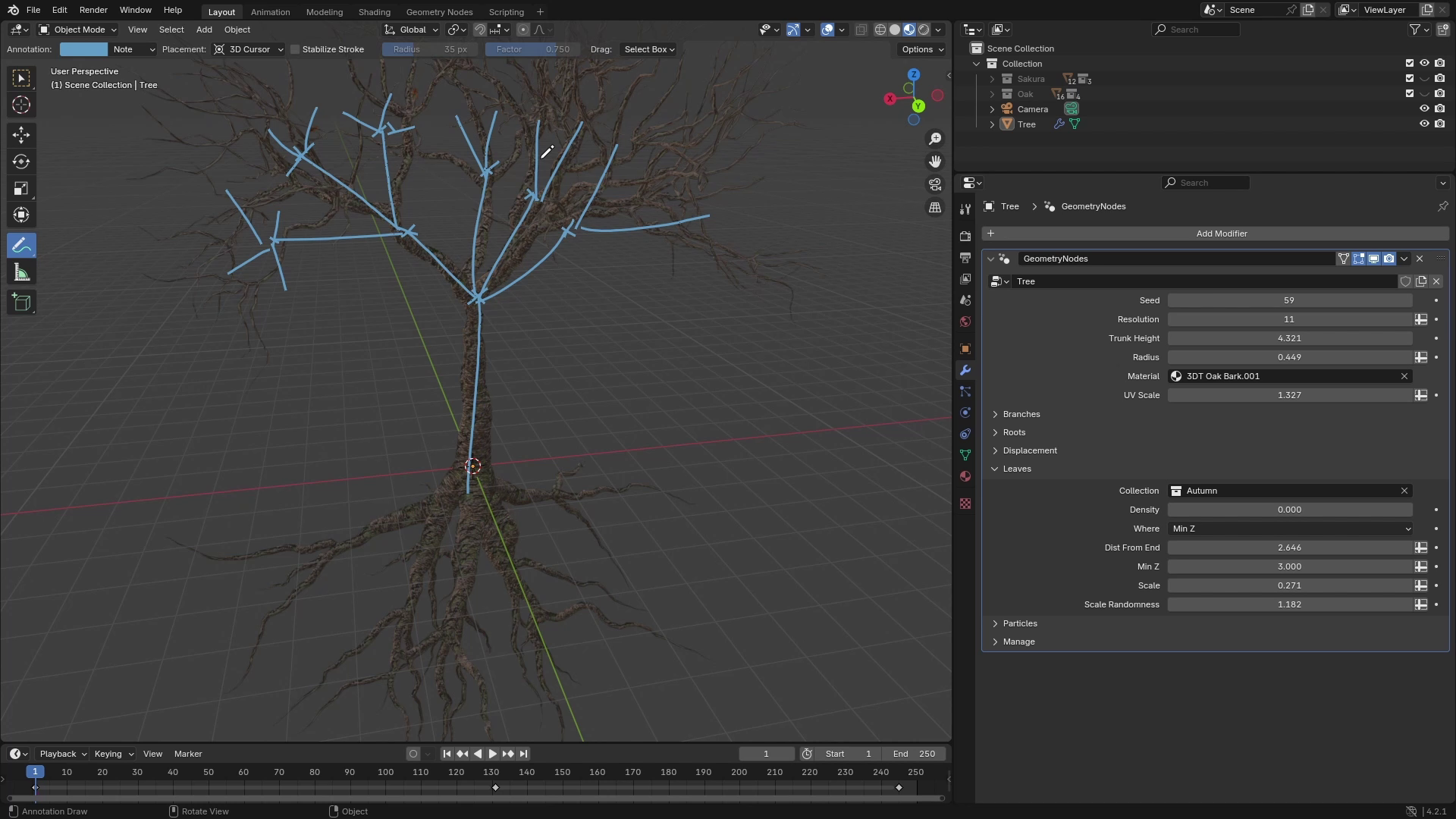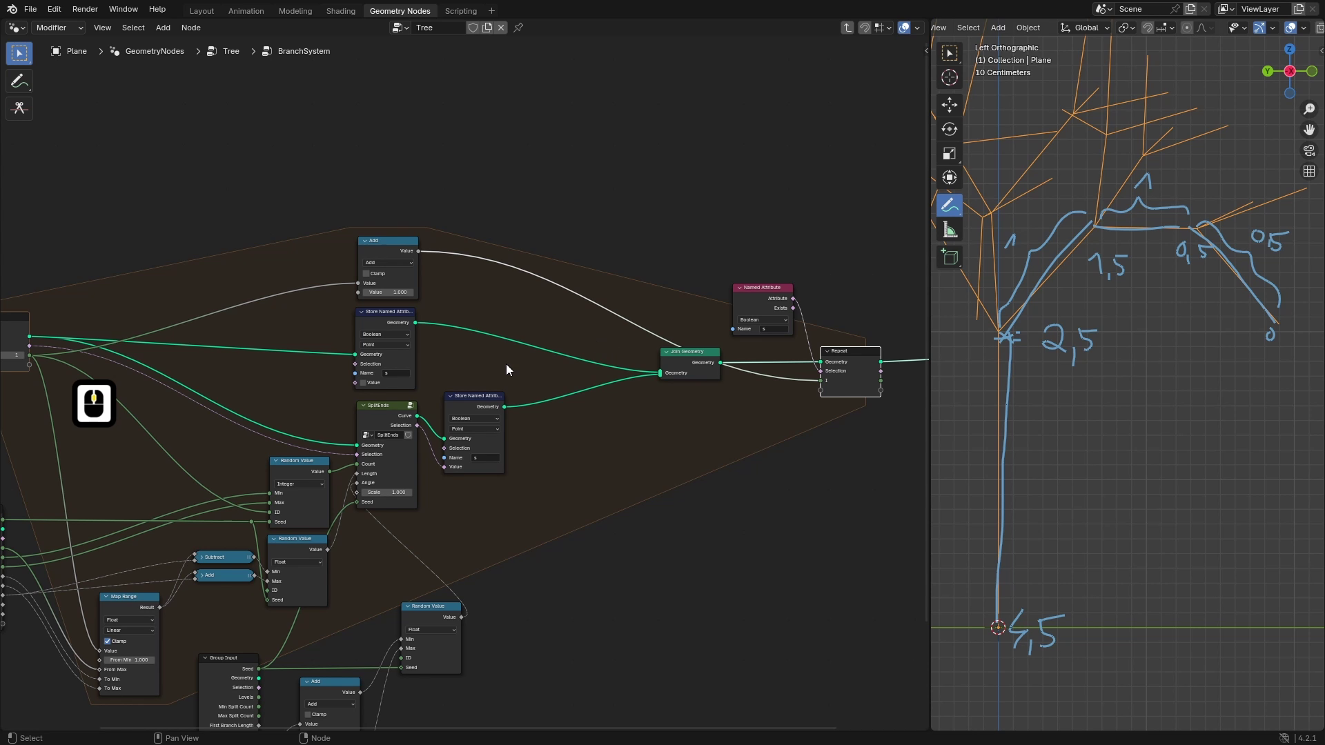3. Branch Generator Intro: Welcome back to three D trees with blender geometry nodes. In this lesson, I'll explain the techniques which we'll be using for generating the branch system and how we'll be able to control it with different perimeters. First, I'll just set density of leaves to zero so we can better see the branch system. And as you can see, we can simplify the structure to just lines. So for example, one main line is the trunk, then there are for branches to which it splits, and then it basically does the same thing at the ends of these branches. So the setup which we will be making will have one input for the geometry. So in this case, when we have trunk, we will give this trunk to this node group, and we will also give it a selection from which we want the branches to grow. So I'll selected with this cross. And what the setup will do is it will just generate branches like this depending on the inputs. So we'll be able to control to how many branches it splits and also how long and angled these branches are. And the output of this node group will be those branches. And also with selections, which will select those endpoints. And then we will use recursive approach or something very similar to recursion, and that we will again use this setup after this first iteration, and this set up will again create some more branches like this. And if we iterate this, for example, three or four times, we should get a nice branch system, which we will use as a basic structure for our geometry nodes modifier. Later in this course, we will also need some attributes for information about the branches. The two main attributes which you'll need is length, and the length will tell us how far each point of the branch is from the roots. So here at the bottom, zero. Here in this section, it's, let's say, for example, two, here it's free everywhere, and here at the ends, it can be like 3.5. With this attribute, we'll be able to control the radius of the branches and also get nice UV maps for them. And the second perimeter will be length from end. And this perimeter will be almost the same as the length, but it will go in different direction or in the opposite direction. So at the ends of the branches, it will be all zeros. And then as we go towards the roots, it will increase. So 0.5 will be here, 1.5 here, 2.5 here, and 3.5 in the roots. With this second attribute, we'll be able to, for example, distribute leaves from ends as I showed in previous lesson, and we will just separate those branches where the length from end is less than some value, and then we can distribute easily leaves on these branches. 4. Split Ends: Welcome back to three D trees with Blender Geometri nodes. In this lesson, we will start working on the foundation of our geometro nodes modifier, and we'll be working on branch system node group, which will help us create the basic branch structure. So here I have a fresh blender scene, and I'll start by deleting everything in the scene. And I'll add, for example, simple plane because we won't be using the original geometry, so you can add whatever you want. Then I'll go to modifiers and add a new modifier, which will be geometry nodes. I'll hit new and call this geometry node setup, for example, three. And now we can start working on the setup. So let's go to Geomet nodes workspace, and we can start by deleting the group input because we won't need this object. The plan for the branches is that first, we will create a basic tree structure from curve lines, so it will look something like this. And then we will convert these curves to mesh using curve to mesh node. So the basic line or the basic curve line will be the trunk. So let's add a curve line and this curve line has two inputs. It has start and end. We can leave start as it is because we want it to start at 00, and the end will control basically the height of the trunk. So if we take a look at the trunk now, you can see that its length is controlled by this Z value of the end vector. So we can separate those values by using Combine XYZ, and now we can control this Z value individually. For the tranghd, we can add a new group input. So let's hit N to bring up this site menu. And I'll click this plus icon to add a new input, which I'll call Trangight we can set the default value to, for example, three and minimum to zero. Now to connect this, we can bring up group input, and we will connect this trunk height to the Z value. You can see that it's zero, so I'll go back to group input to modifier, and now you can see that we can control the height of the curve line with this input. There's also this little warning, and that's because the input geometry must be at the top, so I'll just move it at the top, and now we should be fine. So now we are basically done with the trunk for now and we can just select all of these nodes, hit Control J to bring up the frame, and I'll call this frame a trunk. Now let's start with the node group, which will split a point into more branches. So let's create a new node group. I'll do it by creating a re route to this connection, so I'll hold shift right click and drag over this selection. By the way, if you are not using a node wrangular add on, I really recommend it because it will speed up your workflow in geometry nodes and also the shading nodes. So again, we can do Shift right mouse button and drag, and we can get this readout. And now, if you have this reroute selected, you can press Control G to create a node group. Now if we hit tab, we are outside of this node group, and you can see that it just has one input and one curve output. I will rename this to split ends because it will split end points of the curves. And to go back to this node group, we can again hit tab and we are inside Node group. This node group will have few inputs. First of them is the geometry, which we already have here, but I'll rename it to geometry. The second one will be selection, which will select the points on which we want new branches to grow. So I'll get a new input and call it selection. Type of it will be bullying. And the last for now will be count, which will be a number of branches which you want to generate. So let's add a new input, which will be count, type can be integer, and we can set default to, for example, three and minimum to zero. Now if we go out of this node group by using tab, we will input some basic data to this node group. So first, we will, for example, want to create three branches. So let's add count to three. And for the selection, we only want to grow these branches from this endpoint. So usually the curve line has only two points where the start has index of zero and the end has index of one. So we can just use the index value and where it's equal, so we'll add equal to one. This should select only this endpoint. We can check it with a viewer, so control shift and leftmost button click. This will bring up the viewer, and now we can drag this bullying value to it. And here you can see that this bottom is black and the top one is white. The second method is to check it with attribute text. So here at the top, you can select attribute text, and you can see that here is one and here is zero. So now we have selection done, and let's go back to the node group. We will start by generating a basic branches. So let's add a curve line which will create a branches. And this curve line can be, for example, just 1 meter long. We want to duplicate this curve line depending on this count input, and we can do it, for example, by creating points. So let's add points, and we will create as many points as we want branches. So I'll plug this count into this count. And now you can see that we have three points here. Now to replace the points with the curves, we can use instance on points. And the input points will be the free points in our case, and the instance which we want to replace points with is the curve line. Now, if we view this instances output, you can see that we have three instances. But here in the viewport, you can see that there is still only one line, and that's because they are overlapping each other. So to differentiate between them a little bit, I will first move them on the x axis so they are angled a little bit. And I will also play around with this rotation. So we will rotate it around Z axis depending on their index. So they will be nicely distributed around the Z axis. To do this, I'll add combine XYZ because we only want to control the Z value of this rotation. I'll plug this vector to rotation. Now if we play around with the Z value, you can see that it's rotating around the Z axis. We want different value for each curve, and to differentiate between the curves, we can use index input. So let's add index. And if we plug this index right into the Z axis, you can see that it does something, and that's because for the first line, the input is zero, for the second line, the input, sorry, the index is one, and for the third line, the index is two. We want to distribute those lines evenly in circle, for example, like this. So when we have three curves, we want them to be like this. So between them, it's angle 120 degrees. And to calculate this angle, we can just take a full rotation, which is 360 and divide it by number of branches. So let's do that. I'll duplicate this group input and add a meth node. And because we are using radians here, we will need to use two Pi instead of 360 degrees. So we will be dividing two times Pi, which is 6.28 by the number of branches. And this will give us the angle between each branch. And to distribute them nicely, we can multiply the index by this offset angle. So let's add a multiply and plug it into the Z coordinate. Now you can see that the branches are nicely rotated along the Z axis, and they are nicely distributed around the circle. If we go out of this node group and increase discount, you can see that it works nicely. Let's replace the old approach to rotation with something a little bit better. So I'll set this curve line 0.2 001. Now they are again overlapping. But now if we play around with the rotation on the Y axis, you can see that they are rotating nicely and we can control the angle between branches and the Z axis. So we are basically controlling this angle with this value. We want to control this value from outside. So to add a new input, we can take this empty socket and plug it into Y axis, and I'll bring up the site menu and rename it to angle. We can also set sub type to angle, so the unit in the modifier is in degrees, and the default value can be something like 0.5 or something close to it. Now, if we go back from the node group, you can see that we can control the angle in degrees and also the count. So the next thing you would probably want to control is the length of these branches. But we'll actually do this later because now we should actually distribute those branches on the source points to see how it actually looks like. So let's use this source geometry. And we will use those instances again and instance them on the selected points. So we can actually duplicate this instance on points, and we want to instance on source geometry only where the selection is selected. So let's also plug the selection into it. And as a instances, we want to use this structure which we built from the curve lines. So I'll also plug the instances into this one. And now if I zoom out a little bit, you can see that we have some branches here. And if I go to main geometry node group, you can see that we have the trunk and the sorry, and the first level of branches. And now what we also need is to output the endpoints of these branches because we will want to use the split ends again like this and just reuse this geometry as a new source points. So to get the selection, we can first just realize all of those instances, and then those are again, the curve lines, so we can just take the points where index is one and use this as a selection. To get the index of each point inside the curve, we will want to use a spline perimeter, which will give us index in them. If we use the viewer, you can see that all of the ends of the points have one and the source points have zero. If we would use a index, we would get different values because this index is across all of those splines or curves, and that's not what we want. So we'll just use this pline perimeter index. To make a selection, we can just use a equal and where it's equal to one, this will be our selection. We can plug this result into the group output and rename it to selection. 5. Branch System Basics: Hi, and welcome back to three D trees with Blender geometon rods. Now, if we go out of this split ends, we can duplicate this node group and connect these output curves and selection. And now you can see that this created a second level of the branches. If we use joint geometry and join all of these parts together, you will see that we have a very basic tree structure, which looks pretty cool, but there are still many things which we need to add to the split ends. So first of it, you can see that those branches should be aligned to this curve, so it should look something like this, and they shouldn't be straight towards the Z axis, but they should be aligned to the source curve. So to do this, we can go to split ends, and we'll be controlling the rotation of those curve line chunks. And to get the right rotation, we basically want to align those to the tangent of the source curves. If we look at this from the side. So for example, this step, this is the source curve, and its tangent is vector pointing in this direction. And we want to align the Z axis of this group of curves to this curve tangent, so it will look something like this. For this alignment, we can use align rotation to vector, which does exactly what I drew here. And we want to align Z axis, so that's here selected to this vector. This vector will be the curve tangent, so let's bring up the curve tangent. And this should give us the right rotation. So let's plug this rotation into this rotation. And now you can see that the branches are correctly rotated along the tangents of the source curves. Now when we have this done, we can actually add a length input, which will control the lengths of those branches. So let's bring up the site menu and add a new input, which we will call length. And the default value can be, for example, one. First location where you can control the length of the curves is this one because here we control the basic curve line, and we can just basically control the length of these. The problem with this one is that all of the curves would have same length, and we want to have some variations and randomness in our tree, and this wouldn't look really natural, so we will avoid this one. The second place where we can control this is basically the scale. So if I play around with those values, we can also control length of the curves here. And we can even input different values for different lines, as you can see here is rectangular input, which means there are fields, and we can input a different value for each of them. But if I now at a random value here, and something 1-2. I'm not sure if it will be really visible, but if we maybe decrease the count to three. Yeah, in this one, you can see it nicely. You can see that it almost looks like it works, but those parts here at the second level are all the same, and they are just differently rotated. Want to have as many random things as we can. So to make this even more random, we will use a different approach. You can see that those parts here, here and here, those are the shortest parts, and they are all the same. So to make this even more random, we will do it after realizing the instances and we will move the endpoints of the curves randomly. You can stick to this solution here, but I'll show you even better solution which will give us more randomness. 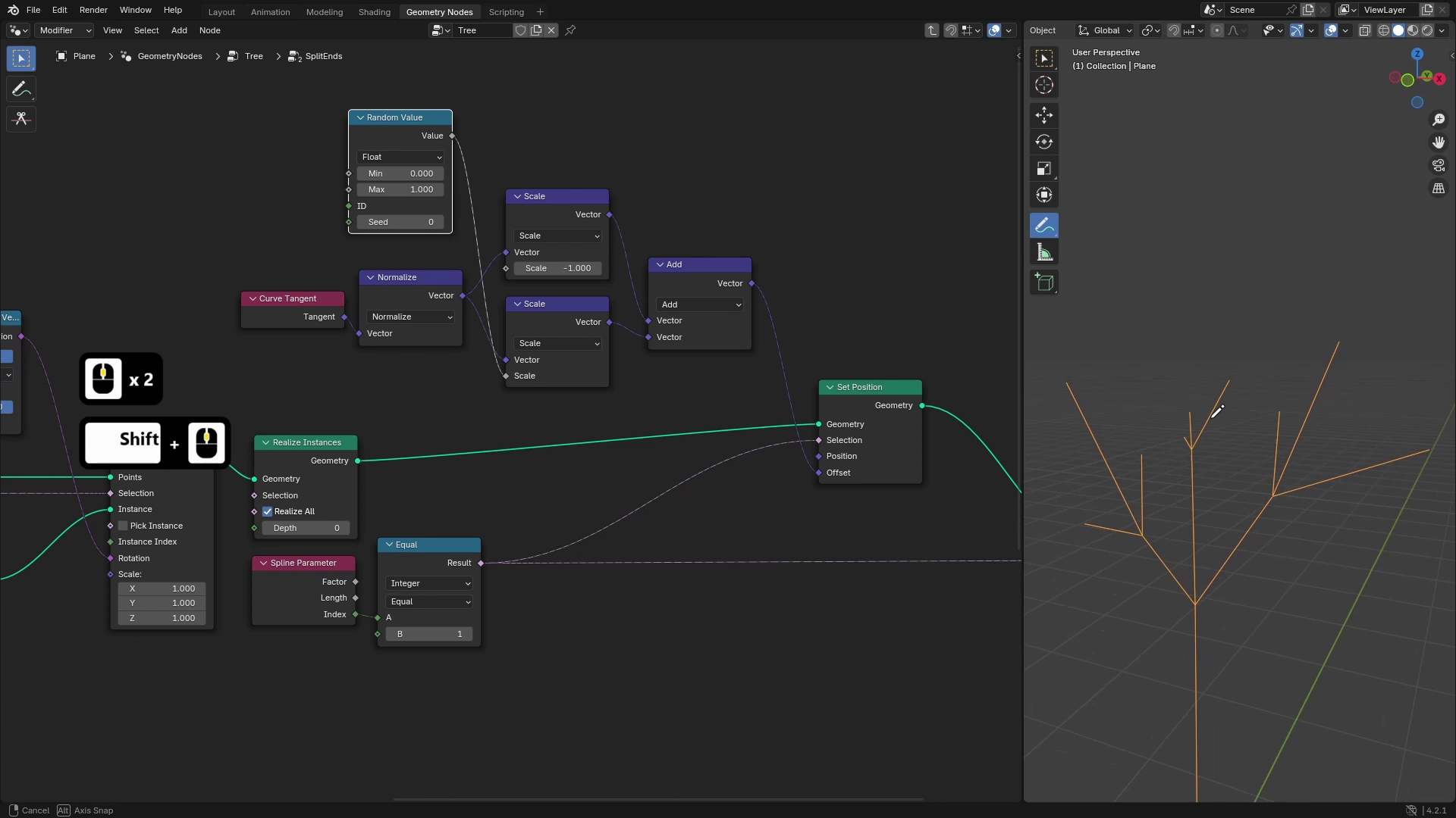So let's delete this one at scale back to one. And now the thing we will do is we will take the endpoints of these curves and move them randomly along their tangent. To do this, let's add a set position note. And we will be only moving the endpoints so we can actually use this selection. So let's plug this into selection. And now if I move it, for example, on Xxs, you can see that it's moving all of the branches, which means that we can control those endpoints separately. The way we will randomize this is that we will get a tangent of each branch and then just randomize it in some range to make it nicer. So first, now we know that those points are 1 meter from their source. So this is one because this end point is on Z axis one. So first, let's reset those points back to those source points and then pick random value in the direction of curve tangent to displace them back. So let's add a curve tangent. And first, we can normalize this, even though this is probably normalized, we'll normalize it. And then if we scale this and plug it into offset, you'll see that we can control length of these curves. If we set it to zero, they have same length as before. If we set it to negative one, you can see that they all collapse into one point. Now, if we add value to this vector, we can control the length of it using the same technique. So let's duplicate the scale value and add it to this original. And we'll plug this result into the offset. Now if we set it to zero, you can see that all of the branches have length zero. And as I increase it, for example, to one, they are back to the original position, but now the controls make actually sense. So when it's one, their length is one, and when I set it to two, their length is two. The nice thing is that there is rectangular control. So there are fields and we can control each branch separately. So if I now plug a random value into this one like this, you will see that those branches have different values or different lengths. You can see that there's this short one and you can't find this short one in the different parts, so you can see that it's truly random. So now to control this input, we can just use the length input which we created and connect it to scale. By default, you can see that it's zero, but now we can control those lengths. And from here, we are also able to plug a random value into it and you can see that it works for all curves separately. The last thing which you would like to add to this node group is to randomize a little bit this distribution in circle because in some cases, this doesn't look real good. For example, if there are only two, you can see that it's straight like this, it's straight, and we want to randomize this a little bit. So let's go to split and node group, and we control this rotation on Z axis here, this combine XYZ in this Z socit. To randomize it a little bit, we will add a value to this. So let's add a add node, and we will be adding to the original value. Now if I plug it into Z axis, you can see that we can basically control the rotation here. We want the rotation to be different for each curve. So we'll use a random value. And if I plug it here, we want this to be, for example, between negative one and positive one. And we also want different seat for each of them. So as a seat, we can, for example, use index of these, and now you can see that they are different. In some cases, what could happen is that all of the branches would be at the same position. So let's say we have three branches like this, and they can rotate like in this direction and direction. So this could end up something like this. So the way to remove this one is that we will limit this randomness in some parts. So basically, we will limit this branch in this part, this branch in this part, and this brand is this third part. So the values we want to input to the random value are basically the offset angle divided by two. So this will give us this angle, and we will just multiply it by negative and positive one, and this will give us the range. So this division here gives us this whole angle, and we will first divide it by two to get half of it, and then we can multiply it by positive and negative 0.5, which should give us those limiting values. Now, if we plug those values into minimum and maximum of this randomness, you'll see that it works nicely. And we can also increase the count. And if we look from the top, you can see they are nicely randomized. To make this a little bit more narrow, for example, we can even divide it by three to get more narrow limits, and I think I'll leave it on freeze so they can be touching each other. All right, the last part is that we'll be adding a seed to this node group because we want to be able to control set of all of these random values. So let's add a new input and connect it to this ID. And I'll just add read out here, and we will rename this ID to seat. Let's also not hide this value, so uncheck this height value because that's by default for the ID. And now we can control it from outside, so you can see that we can control the randomness of the rotation on first level and also the second level. To test this, let's also at the third level. I'll again, use the previous curves and selection, and I'll join it into the spin and we can make this a little shorter. You can see that we have now a pretty interesting structure, which looks a little bit like tree. But in the next lessons, we'll add more details, which will make this even better. 6. Advanced Branch System: Welcome back to free D trees with blender geometry nodes. In this lesson, we will continue working on our branch system, and specifically, we will create a new node group which will combine those split ends and create a complete branch system. So first, let's delete those nodes because we won't need them anymore, and we will create a new node group. So I'll just connect this curve to output geometry at a rearut and with selected rear out, I'll hit Control G to create a new node group. 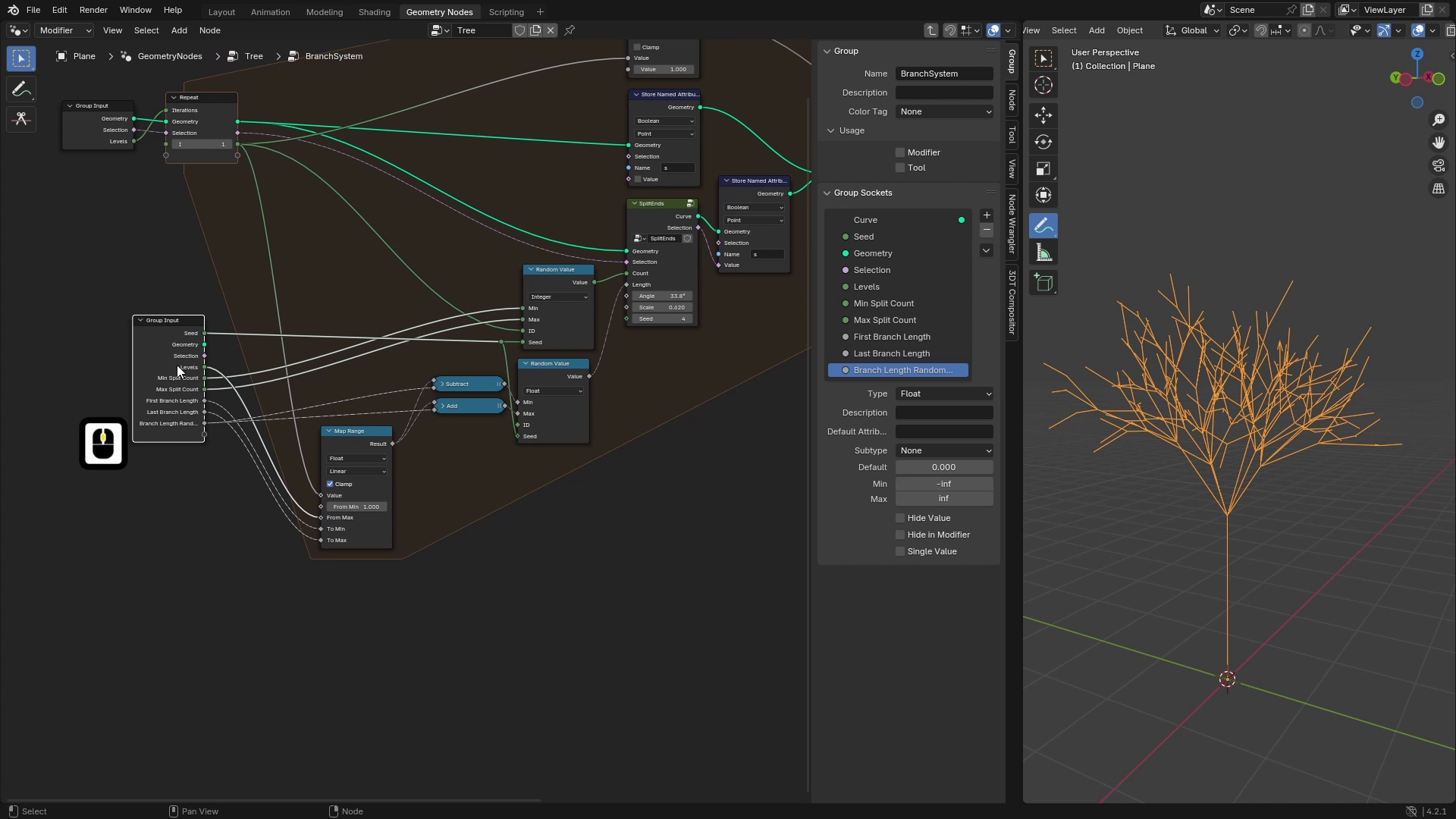I'll call this node group a branch system. So how this branch system node group will work is that it will have a few inputs. One of them will be selection, which will be the point from which we want to grow the branches. So let's say this is the trunk and this is the selection, and then we will plug it into Branch system. Input which will be in branch system is number of levels. So that is number of levels of branches. So for example, this is how two levels of branches look like, and if we add one more, this is three levels. So we'll be able to control how many levels there are. And later we will also add some kind of randomization. So there will be length of first branches and last branches, and it will interpate between those values and also how much the branches will split. So there will be minimal and maximal number of branches which will be generated on each so let's go into branch system node group and add some of the inputs. First one will be selection. So I'll add a new bullying input and call it selection. And the next important one is number of levels. So let's add a new input. This one will be integer, and we can call it levels. I think this is fine for now and we can start working on overall setup. So let's add our split ends node group, which will be the base of this node group. And basically how this will work is that we will use a repeat zone, which will have split ends inside of it, and the repeat zone will iterate depending on number of levels which we input to this node group. And after all of those iterations, it will create a final branch system. So let's add a repeat zone. And number of iterations will be levels, so we can plug levels into iterations, and output geometry will come from the stripe zone so we can plug this into output. The starting geometry will be the trunk which we input to this node group, so we can also plug the geometry into this geometry. And on each iteration, we will use this geometry, so we can plug this into split ends. We've given selection and join it with the previous geometry. So let's add chin geometry, and we will join it into the source geometry, basically. And we also need to store the selection. So let's plug this selection into this empty socket, which will create a new socket here with selection, and we will use this one as a selection for next iteration. So for the first iteration, this will be selection from group input. But later in next iterations, we want to use selection from those new branches. So we'll plug this into the output. Now if we go outside of this node group and increase number of levels, you can see that it starts growing. I'll also play around with the count, and you can see that we can control how many levels of branches there are. If we now check how many curves there actually are, you can see there are 16 splines, but that doesn't correspond with what we see because if we count this, we have one trunk, three branches, and each of them has three second level branches, which should add up to 13, but we have 16. The problem here is that this selection doesn't delete the previous selection. So to actually fix this selection, we will create a new named attribute, and that will tell us which points we want to expand in next iteration. And for old geometry, we will set it to falls, and for new geometry, we will set it to the selection. So let's add a store named attribute. And we can call it as for selection, the type will be Bolin, and for all of those branches from previous levels, this will be false. So we'll leave this on falls. And if we duplicate this and plug it into those split ends, we'll plug selection to the value. And now for the selection in next iteration, we can use this named attribute called S and plug it into the selection. Now if we increase the levels to two, you can see that we only have 13 splines down instead of 16. So that's working nicely. And now we can start working on connecting those inputs from split ends to this group input. So the next input of the split ends is count, and we actually want to randomize this input because we don't want it to be constant, but we want some variations here. So, for example, the first level would split into three branches, then four and then only two or something like that. So to do that, we will add a random value The type of this random value will be integers because count is also integer, and we'll plug those minimum and maximum values into group inputs. So we can use this empty gray circuit to connect it, and this output value will be plugged into count. You can see that now this connection is red, but we can fix this we can add a new variable into this repeat zone, which will tell us in which iteration we will be. And if we plug this iteration into ID or C, this will converge to constant and not a field value, and this shouldn't be read anymore. So we've selected repeat zone, hit N, and go to node, and we will add a new input, which I'll call I as iteration and set type two integer. And at the start, we want it to be, for example, zero, and then in each iteration, we want to increase this by one. So let's add at math we will add one to it and store it for the next iteration. Now this will be incrementing every iteration. So that means it will be different for each iteration, and we can use it, for example, for ID, and now you can see that the value isn't filled anymore. And that created something strange, but that's because the minimum is zero and maximum is 100. If we change this to let's say, two to five, you can see that on first iteration, this split it to five branches and on the next one only 23. We also want to be able to control the seed. So let's also connect the seed to the group input. And I'll just rename those Min and max to Min split count and max split count. And also move set to the top of the group input as always. So now the number of levels is randomized and the next input is length. Further length, we will also create some randomization, so we can duplicate this random value and set it to float. And if we now plug this random value into this length, you will see that each of the branches have different length, and that's what we exactly want. For the sad, we can plug the seat from group input to this seed and we can leave ID as it is because by default, it picks index, which is fine for this purpose. For the min and max values, there are few options how we can control this. And one thing I would like to do is I want to make this dependent on the current level of iteration on which we are. So we'll be able to create, for example, long branches in first level and then shorter branches on the last level. And we will also want to randomize these a little bit, so we will add some kind of randomness. So let's add a first input, which will be first branch length, which will set a length of branches on first level, and we can set default to one and minimum to zero. And I'll duplicate this and rename this to last branch length, which will control the length of last branches or basically branches in last level and set it, for example, to 0.5. The last input for the branches will be branch length randomness, so let's add that as well. And we can leave those default values as they are. So now to calculate length of branch on each level, we will use a map wrench and also this I value which we used for ID for the randomization. So let's add a map wrench. And we will be remapping this I because it's going from zero to number of levels minus one. Or in this case, we can actually increase it to the starting value to one, and now this will go from one to number of levels. And now we can just remap this I value with map wrench from one to number of levels. And the range to which we want to remap this will be from first branch length to last branch length. This means that when the I is one, which means we are on the first level, the output of this map branch will be first branch length. And if we are on the last level, which is where the I is levels, the length of branches will be last branch length. We will use this value for the randomization, and the way we will randomize this is that we will add a random value to this base length in range of minus randomness and plus randomness. Basically, if I visualize this, let's say here is this map range value and we will randomize it in a range where this is L minus randomness, and this is L plus randomness. So if the R is something small, it will be in a small range between the L, and if it's larger, it will have more variations. So that means that the minimum of this random value will be this map ranch minus branch line randomness. So let's subtract this from the map ranch. And the maximum will be map wrench plus randomness, so I can duplicate this with Control Shi D and just change type to addition. Now, if we plug those to minimum and maximum and go outside, you can see that we can control the levels depending on their level. And if I increase the levels, you will see that if I change first branch length, it's only changing the first level and also the other ones, but the biggest change is on the first level, and we can also control the last branch length as well as branch randomness. Right, so now I think the branch system is ready for the next usage. We can also play around with the inputs, and you can see that it's generating pretty nice three structures. And the last thing which we can do is we can connect those inputs to the main group input and also create a panel which will control the branches. So let's add a new panel. I'll collate branches. And now I will bring up a group input, and as always, use this empty socket to create those new inputs. And because if we connect this to the socket, it will use the current value as a default. So I'll just set some nice default values here. So something like this. And now I will create all of those inputs in the group input by just dragging this empty circuit into all of them. When all of the inputs are created, I'll just move them into dright panel, which is the branches panel. And I'll also move seed to the top of the inputs and hide those on sockets with Control H, for example, now it's looking pretty good. One more thing which we might do is clean up this tree a little bit. So I'll just use different group input. So this isn't that messy. And just reconnect those inputs to their own group inputs. Now, when everything is finished, we can go to modifier step, and you can play around with this basic tree structure with all of those inputs. One last thing which I forgot to add is controlling the angle because we forget to this one. And with this angle, we want to control, actually, how spread the overall branch system is. So let's also quickly add a new inputs for these for this, we will just pick a base angle and then the randomness, and it will work the same way as the branch length, but just with one basic angle. So let's add first input to angle and second one to angle randomness. I'll duplicate this group input, and we'll use the same technique as here. So I'll just use this random value, use this one, this sat, and we'll just add and subtract the randomness from basic value like this and plug it into minimum and maximum values. This will generate the random angle, and we can plug it into the angle. You can see that now it's all flat, but that's because those inputs are set to zero, so I'll just increase it a little bit. And we can also set the sub type of these two angle so they are in degrees. The last thing which we should do is connect this seed to our global seed. So I'll just connect seed from group input to split ends. And to finish it, we will connect those two inputs to the global group input, again, with this gray, sock it and move them into branches panel. 7. Internal Data: Hello, and welcome back to free D trees with blender geometon nodes. In this lesson, we will implement internal data which we will be using for distributing our leaves and also fingering out radius of each branch for each point. I have already explained those data in introduction to branches, but I'll shortly go through them. Both of those will be attributes which will be stored for each point, and first of them is length. Which at the start of the root is zero, and then it increases depending on how far from the root we are. So, for example, it can look something like this. And then we will also implement the inversion of this or opposite version, which will be called length from end. And this one will be the same, but in the opposite direction. So at the ends of the branches, this will be zero. And as we get closer to the root, the value will be increasing. The length from end will be used for distributing the leaves at the ends of the branches. So for example, we can set the value to zero point or 1.5, which can be somewhere here, and the leaves will be only distributed at these branches. And the basic length will be used for calculating the radius of the branch mesh. Alright, so let's get into geometry nodes, and we'll be implementing both of those inside branch system. So let's go to branch system. And the first one which we want to use is the length because that one will be a little bit simpler. So we'll be storing those attributes. So first one, we can actually store some basic length for the trunk. So I'll add Sterne attribute. It will be float for each point, so the default values are fine, and the name will be length. For this one, we will use a spline perimeter, which will give us length of each point. And if we visualize this, you can see that it's zero at the bottom and two at the top. Now if we go to branch system, the way this will work is that, for example, in this first level, I'll just decrease this. In this first level, this source point has length of two. For all of those points, we will add a length to this basic value, and this will give us, for example, if this curve has length of one, it will create three at this point. So the length will be implemented inside the split ends because we can do it here. So I'll go to split ends and we will be storing here at the end after displacing the end points depending on the length. So I'll add a store named attribute, set name to length. And the length will be the current length of the curve plus the length of the source point. So we'll add a value to this one, and the value which we will use is the length of the source point. So we will capture it before instancing the curve on it. So let's add capture attribute. And we will be capturing the length. So let's also add named attribute, length. We will capture it like this, and then we will plug this value into this addition, which means that, for example, if this point has two, this curve has length 0-1, those values will add together, and we will get two here at the bottom and three here at the top. So if we store this into named attribute, we can now visualize this at the end of this repeat zone, so I'll bring up named attribute. And now you can see that those points have a little different values. Maybe I'll visualize this at the end of this branch system that will be the best. And we can also increase number of levels and make the branches more visible. Now if we visualize this, you can see that this source point has attribute length zero, then this value is somewhere around three. And there's 3.7, 4.7. All right, I think I made a little mistake inside the split ends. Here in the addition, there must be this spline perimeter and the spine length, which I used before because this spine length will give us only the length of the curve, but we want length on each point. So we need to use this spin perimeter. And now if we visualize those values, with the greater then, for example, so I'll at greater then and disable this attribute text. You can see that as I increase this value, all of the branches get black, and to make this even more visible, we can resample those curves to more points, and now you will see this nice border between black and white, which is going along the branches. So that's for the length. Now we want the opposite attribute which is length from end. This one will be a little bit trickier, and that's because the way we build the branch system is that we start from the trunk and then continue to ends. But the best scenario would be that we would start from the ends and then go to start, but that's a little that will be very complicated. So we need to figure out a way to calculate the length from the ends. The way we will calculate this is that for the trunk, we will store the length in opposite direction, so length from end. So at the top, it will be zero, and at the bottom, it's two because this one will be the end. And here at the bottom, the length from end is two. And then on each iteration, we will take the length of the next branch. So let's say this one is one and add it to all of those points. So this one will be zero plus one and two plus one. And for this curve, we will again store the inverted length from end. So here will be zero, and here will be one, which corresponds to this one. Now, if we do this for each level, again, this one has one and we will edit at this length to all of the previous points. So this one will be two. This one will be one, and this is two plus one plus one, which is four. And you can see that this in each level, it builds up the distance from end. And let's say this is 0.5, it'll be zero, 0.5, one plus five, 2.5 and 4.5 and you can see that at the end, we should have this value which corresponds to length from end. We will also implement this inside branch system, but we won't go into split ends, but we also stay here in the repeat zone. And as before, we will first start by storing this attribute for the main trunk. So let's use another named attribute, but we'll call this one length from end. And this one will be inverted length. So to get the inverted length, we can take the overall length of this curve and then subtract this perimeter from it. So let's also at sorry, spine length, which will give us the length of the curve. You will subtract this length perimeter, which is going from zero to length for each point and start for the length from end. If we visualize this value, you can see that it's zero here at the top and two here at the bottom. Now in branch system, we'll do exactly what I explained here. So for those new curves, we will just store the inverted length. So I'll again, use this surnamed attribute, set it to length from end. The type will be flowed, and we will use the same value as we used here. So we will take a spline length and subtract the spline perimeter Like this. This will again give us the inverted length factor, and we'll store in length from end. And for all of the previous levels which is this socket, we will add a maximum length of these nu curves to their length from end. So I'll duplicate this one and we will take their previous length from end, which we'll take with named attribute and add a length of these curves to this length. The problem here is that those new curves might have different lengths, and there isn't really a way to get each different length to the previous levels. Let's say we have the strunk and then it generates two branches. One is shorter and one is longer. So this previous level has, let's say, here is one and here is zero, and we can't figure out the length in this point because from this point, it's I don't know, let's say, 0.2, but from this end, it can be like one. So we don't know which value we want here. And in my opinion, the best thing to do is we can add or we can add the maximum length of these curves. So because this is 0.2 and this one is one, we'll use this curve which means that this point will have distance one, and this will have one plus one, which is two. So to get this maximum length, we can just take this geometry and use attribute statistics. And we will want the maximum length of the curves. So the domain in which we'll select will be spine, and the attribute we want to use is this length from spine length. So I'll duplicate it and plug it into attribute and make some space here. And basically, we'll just take this maximum and add it to the previous length from end like this and store it into length from end. So to sum it up, for the new curves, we will store the inverted length factor, and for the old curves, we will just add a maximum length of these new curves to their previous length from end. Now, if we visualize this here, I'll again use named attribute length from end. It's here. And we can again use the greater then because with that, we can nicely visualize this. And as I increase this, you can see that this value nicely goes from the ends of the branches to the root. You can see that if it's zero, all of them are white, and as I increase it, the ends are black, and it's going towards the root. 8. Roots: Welcome back to free D trees with Blender geometry rods. In this lesson, we'll continue working on our tree structure. Specifically, we'll be working on the roots. If you try drawing roots to our tree, so something like this, notice that this shape down here is very similar to this up here. And that's exactly what we will use because we will reuse our branch system node group to create the roots with same technique. So let's go to Geometri nodes, and here we can see that in this part, we are creating our branch system, and we will add the same thing, but for the roots. So for that, we can duplicate this branch system node group. And if we take a look at our trunk, we will be using this one as well, but we don't want to grow branches from the top part but from the bottom part. So let's plug our geometry to geometry here. And if we now output this branch system, we can see anything. But if we put our original selection here, we have a very basic tree, same as before. First thing we need to fix is that we want the branches to grow from the bottom. So instead of point with index one, which is up here, we want to grow them from point with index of zero. So we can duplicate this equal with Control h D and just change one to zero. And where this is equal to zero, it will create the branches. Now you can see that it creates the branches, but there is a problem because they are growing in the wrong direction. We want them to grow in this direction instead of this direction. To fix that, the easiest way to do this is to just take the trunk curve and reverse it, which will reverse the direction of this curve. So let's add reverse curve and plug our trunk to it. And if we now plug this curve into geometry and this selection to the selection of branch system, you can see that the branch system created exactly what we are looking for, and those are the branches which are growing from the bottom of our trunk. Now what we can do, we can combine those generated curves with the branch curves. So I'll just join these geometries together. You can first just add a joint geometry and connect them separately and connect them manually or you can hold Control shift right click and drag over those two nodes like this, and this will generate the joint geometry and join both of these branches together. Now if we output this, you can see that we have a nice tree structure. The only problem now which we have in the setup is that this branch system contains the trunk curve, as well as the root system also contains this trunk curve. So that means that now here in this section, there are two same curves which are overlapping. We don't want something like this, so we need to get rid of one of those trunks. To get rid of one of these trunks, we can, for example, store attribute before all of those node groups for the trunk and then check where this attribute is assigned and we will remove this geometry. So for example, here, we will add a rear route, and we will add a store named attribute. For example, we can add a Bolin, we can call it, for example, trunk and set it to true. This means that now the trunk curve has this trunk attribute assigned. And in the branch system, we will add this attribute as well, but we will set it to falls. So let's go to branch system. And here where we are joining our new branches to the whole setup, we will add a store named attribute, and we will again store the trunk, but set it to falls. Now if we go outside of this branch system and check the named attribute trunk, you can see that this curve is true, but those curves are all false. So we can use that. And for example, I'll delete this trunk from the roots, but you can delete them from branches as well, but only from one of these. So let's add delete geometry, and where the trunk is true, you want to delete it. So I'll use it like this. Now if we view this, you can see that the roots don't contain the trunk, but those branches contain it. So together, it will give us the whole tree without any overlapping. Right. So now our curve system has roots as well, and we want to be able to control all of these parameters, which we can control for branches. We want to control them for roots as well. So for that, we will add a bunch of group inputs, and we'll be adding them with this empty sockit. So for the seat, we can use the one existing. So let's plug it into seat. But this will result that those both node groups will use the same sad, and we might get same results on them. So let's make it a little different. For that, we can, for example, use a MF node. I like to multiply at, and we will multiply this seed by, for example, 15 and at some random number, let's say 42. And now this will probably give us always the different sad than the original value. So now we have the seat, and now we will just connect all of these group inputs or sockets to the group input. So we will use this empty socket and I'll plug them like this. And now when all of those sockets are connected, we can hit to bring up the site menu, and I'll add a new panel which I'll call roots. To finish it, I'll move all of these attributes or inputs to this roots panel. All right, so now when all of the socits are connected, we can hide a new socuits with Control H and also clean this note tree a little bit. I will just group those nodes with Control J and call it remove duplicated trunk. And we can also rename this whole setup to branch system. Now we can go to Modifier and play around with our roots. So I'll set levels to something smaller and make them a little longer and also play around with the angles. We can also check if both of our attributes which are length and length from end are working correctly. So I'll just add a named attribute and length, and we will check where it's greater than some threshold value, and I'll hide those attribute texts. So as I increase it, you can see that it's going nicely from this point here to the branches, as well as to the roots. And to check the other parameter, which is length from end, you can see that it's also working really nicely. 9. Displacement: Welcome back to three D trees with blender geometry nodes. In this lesson, we'll be working on the displacement of our curve setup, and we will give this tree a little bit more natural look. So how this will work is that basically, we'll just take those curves and we will displace them with some noise textures. But before that, we need to be able to control how much geometry this tree actually have. We'll be controlling it with this resample curve, but we will give user option to control how much resolution we actually have. To do this, it's actually better to switch this type to length because that means that it will sample those curves to evenly distributed points, and it doesn't depend on the length of the curve. And we can add one perimeter to this node group, which will be the resolution. So let's add a new integer input, which will be called resolution. And we can set the default value to, for example, ten and minimum to one. If we bring up the group input, we can't really plug this resolution straight into this resample curve because those integer values are really high, and you can see that it doesn't really work. We want some smaller values here. But for the user, it's better to work with those integer values. So to calculate this length, we can use MF node and we can just divide some constant by this resolution, which means that if we increase this resolution, it will make this division smaller or the result will be smaller, and the geometry will have more points. So if we use 0.5, for example, you can see that now when the resolution is set to one, the steps between the points is 0.5. But if we set it to, for example, ten, the steps between the points will be 0.05. So for now, I will leave it like this, and we can work on the displacement with noise textures. To do this, we will be using a simple set position node. So let's add that. And we'll be using this offset input with which you can offset the tree in all directions. If we now add noise texture, for example, this color outputs three dimensional vector with values 0-1. If we plug this straight into the offset, you can already see that it does some kind of displacement. And if we play around with the scale, you can see that the tree is much nicer now. The problem is that the root of the tree isn't at 000, so that's the first problem, and the whole tree is kind of moved in this direction. That's all because of this color, which gives us only positive vectors, and we also want some negative vectors. To change that, we can use a map range and we can remap this vector because the color is vector from 000111 to negative ones to ones. This will result that this vector will also give us some negative values. And if we plug this into offset, now you can see that the tree is almost centered, and that fixes a little bit. But still, the center isn't exactly at zero, zero, zero. To change that, we can use one of the attributes which we are storing, and that's the length. If we view the length, you can see that the length is zero here at the center or at the root, and it's increasing towards the branches. We can use this value to multiply this vector, which will result into that this point will stay at zero, zero, zero, because if we multiply the vector here by zero, it will be zero. And as we go towards the branches, it will be multiplied by one. So if we take this length and multiply this vector by it, so we can use a scale for that. This will result in something like this. You can see that the branches at the ends are really distorted, but this vector or rose the starting point is still at zero, zero, zero. The branches here are very displaced because the length is much higher. And we want this multipler be one at the maximum. So for that, we can use a clamp which will clamp the value in some range. So if it's higher than the maximum, it will go back to the maximum. So if we clamp this 0-1, you can see that now this looks much better. We can also visualize this, and you can see that this clamp value multiplies those vectors by zero. But when it's somewhere here, they are already the original and they are multiplied by one. So now this looks relatively nice, and we want to be able to control how much those points are distorted. To do this, we can multiply this clamped value by some constant. So let's at multiply. And plug it into scale. Now if I play around with this value, you can see that I can change how much the noise impacts the displacement of the points. The second perimeter, which we can also control is very important is scale of the noise. So if you play around with the noise and make it smaller, you can see that the tree has much smoother distortion. And if we set it to something higher, you can see that it's very harsh and it's very detailed. To get the best results, it's really good to combine few of these noise textures together. So we will combine two of them, and we will want to use them in that way that the first one will have a very low scale, and it will create a displacement like this, so the branches will be very smooth, and then we will apply another noise texture which will have much higher scale and add those harsh details. So we can reuse the setup once more, and we'll just add those values together. The values which we want to control is this multiplication value and this scale. So let's add some group inputs. I'll hit N, and I'll add a new panel which I'll call displacement. And I'll add inputs for this first noise texture. So the first input will be noise scale one and noise power one. And I'll set default to something like 0.25 and power also 0.25, we can try it here how it looks. Maybe that's too small. I'll set power to one. And now for the second texture which you'll be using, we can just duplicate those and I rename them to twos. For this one, I'll use a scale of let's say one, and the noise power two will have a default value. But 0.25, for example. Now let's go to modifier and also reset these to their default values. And we can connect those inputs to this first setup. So I'll bring up group input and connect this noise scale one to scale and noise power one to this multiplication. I want to duplicate the setup, so I'll just select those nodes and hit Control G, and I'll just rename those inputs. This scale is great, and the second one will be Power. And we can call this node group branch displacement. And because we want to add one more displacement, I'll duplicate this and use different scale and different power. To combine these together, we can just add those vectors. So let's add addition and plug this resulting vector into offset. Now, if I go to Modifier, you can see that we can control the impacts of these both textures, and we can get some very interesting results. To ensure that those noise textures aren't the same, we can change this type in noise texture to four D and use this W perimeter, which is something like CT. So I'll plug this W into the group input and just move it up. And now outside of these node groups, I'll use the set. And again, we will get some different values from this seat with multiply Ed node. So let's add multiply ad. So first one, again, we can just use some random values. And I'll apply this first one to this W and the second one you can really just use some random values and they'll probably have different values for each seat. They'll plug this to the second W. We can hide those and also hide a new circuits with Control H. Now, as we change the seat, the seats of the noise textures will change as well. To finish this up, we can select all of these notes and call it displacement. Also this previous part, we can call it resolution. 10. Mesh Generation: Welcome back to three D trees with blender geometric nodes. In this lesson, we will start generating the actual mesh of our tree and also add some basic UV maps. So let's go to Geometri nodes. And the first thing is that to generate a mesh from curves, we will be using a curve to mesh node, so we can add that. And for the profile, we will use a curve circle for now because we want it to be circular. Now, if we plug this curve into profile curve and decrease the radius, you can see that we have not pretty nice, but we have some really basic mesh around our curve structure. For now, we can also check this fill caps so the ends are filled. And the first thing which we'll do is we will play around with the radius of the curve. If we add a set curve radius, you can see that with this note, we can control the radius of each point, and we can control them separately, which is very powerful. So for our tree, we want the radius here at the start to be somewhere around one, for example, and here at the end, we want it to be somewhere around zero, so it will be decreasing as it's going or as it's approaching the ends of the branches. To get this value, we can use our length attribute which we are capturing. So if we visualize our length, you can see that it's zero at here and it's increasing towards the ends of branches. The problem here is that the values are very high. Here at the end is something like 6.9, but the ideal value would be just one, and then we can just flip this attribute. So to remap this length from zero to this 6.9 or what the value is. We can just take the maximum length of these branches and divide the length by this. So for example, if the maximum length at these branches would be seven here at this point will be something like 0.95 or something like that, and that's what we are looking for. So to get the maximum length of these branches, we can use attribute statistics. So let's add attribute statistic note. And we want statistic of this length. So let's plug this length attribute to attribute, and we want to take this maximum. Now to convert this length to range zero to one, we can just divide it by this maximum. And if we now visualize this, you will see that here at the end is something like 0.99, and here at the start, it's somewhere around zero. So that's exactly what we are looking for. The only problem now is that if you take a look at the roots, the values at the ends aren't really one, but they are 0.27 and so on. And that's because the branches here at the top are much longer than the roots. But the roots are using the maximal length of the branches as well. So we need to separate these two parts and calculate this factor separately. For that, we will move this calculation into the branch system, and this will separate those two parts. So I'll just delete those nodes here, and I'll go to branch system, and we can calculate this factor at the end of the repeat zone. So here at the repeat zone, at the end of repeat zone, we will add attribute statistic node and we will take a length attribute. And just divide it by the maximum. So the same thing as we did before. And here we can just store this value in another attribute. So I'll add store named attribute, and I'll call it, for example, length factor, and plug this result into this attribute. Now, if we go back to the end of our setup and visualize this length factor, you can see that now the branches still have 0.99, but the roots also has something around 0.807, and they are very close to one. So that's nice. And for example, now, if we plug this attribute into the radios, you will see that the branches are thin here at the start and thicker towards the ends of branches. We want to flip this and we want the maximum thickness at the start and minimal at the ends. So to flip this, we can just take the math node and subtract this value from one. So something like this. Now you can see that the branches or the root is the thickest part here. And as we go to the end, they are thinner and thinner. Then you can also control the overall radius with the radius of the curve circle, and it's looking pretty nice. Currently, the fall off is linear. So if we draw a graph here, and here on the y axis will be the radius, and on the X axis will be the length factor. I'll just mark it like here. Currently, where the length factor is zero, the radius is one, and where the length factor is one, the radius is zero. So it looks something like this. In some cases, we might want the branches to be thinner earlier in the tree. So we want the curve look something like this. Or on the other hand, we want them to be thicker longer time as we go to the ends. So we want to we want it to look like this. To control this, we might use, for example, float curve where we can do exactly something like this. So if we add a float curve after this one, we can just play around with this value. Now you can see that if I put it under the linear function, you can see that the branches are thinner, and if I put it here, they are thicker. The problem here is that we can't actually control this float curve outside of this node group or outside of this modifier. So we need to get a different way to do this. So the way we will do this is we will use function X to the A where the X is factor or our length factor and the A is input variable which can be controlled by the user. Here it's visualized. So when the A or the exponent is set to one, the function is linear. But if I set it to something lower than one, you can see that the function goes more like this, which means that the branches will be more thicker. And if it's over one, you can see that it's going under the linear function, which means that they'll be thinner. So to implement this into blender, we can just take this value and use a Bower and the exponent will be value 0-2. So if we set it to one, you can see that we have the same results as we get with linear function. If I set it to something smaller than one, they are thicker, and if it's higher than one, you can see that they are thinner. 11. UV Mapping and Refinement: Hi, and welcome back to three D trees with blender geometry rods. You can go even more than two, and you get even nicer gradient. But that's up to, I will probably set maximum value to something like three and leave it like this. So to add some controls, I'll bring up the site menu, and the first thing which I'll add is the overall radius. Which will be controlling radius of this curve circle. I'll set default value to 0.15, and the second one will be radius fall off, which will be this exponent. So I'll add a new input and call it radius fall off. The subtype, I'll set it to actor because it will be in small range, so you can use that. Set Default to one and set it 0-3. To use these group inputs, I'll just connect them from the group input. Also the radius to the curve circle. Now, if I go to modifier, you can see that now I can control the radius of these curves and their fall off. We could also set those values separately for branches and roots. Then the best way would be to put those controls into the branch system as well, but I'll just stick to this version. So to clean this up a little bit, I'll just move this radius here and now we can call this group of nodes radius because we are controlling radius here. Now the next thing which we are not controlling yet is this resolution. One way would be to just edit to the group input, but we can do it a little bit smarter. We can just use this resolution input, which we already have and just calculate how many points the curve circle should have. So for the resolution, we are calculating here. And with this division, we get offset between two points. So I'll just duplicate this with Shift D and parent with TP, so it's not inside the frame and just move it here to the front. And basically, the curve circle looks like this, and we know what radius it has. So we know this R value, and we need to calculate how many points it will have. The information we also know is the spacing between the points this division. So we know, I'll just draw a bunch of points here, something like this. And we know how long this gap should be. Let's call it G as gap. And to calculate the number of points which fit in here, we can just use that the length of the circle is two by times radius. This will give us the whole length. And if we divide it by this gap, we should get the number of points which we need to create. So let's calculate this. I will just multiply this radius by two Pi like this and then just divide it by this gap value, which is here. And if you plug this into resolution, you will see that the value we get is 17.6, it automatically rounds, so we don't need to round this value. And now if we take a look at the geometry and for example, decrease the resolution, you can also see that it decreases number of points automatically, and we don't need to worry about it. All right, so the last part will be generating the UVs. To generate the UV map, we will need two variables. One of them will be increasing towards the ends of branches, and the second one of them will need to go around the branches, and this will generate our texture coordinates. So first, for this one, we can just use our length attribute because we have this already calculated, and it should be correctly calculated. So we can just use this one. And for the second axis, we can use a factor of this curve which you are using for the profile. So if you look at this circle and use a plain perimeter, which includes the factor, you can see that this factor is going 0-1 around the circle, and we can use this value for the UV. So we need to capture this attribute using before generating the mesh. So let's add capture attribute, and we will want to capture this factor for each point. And now after the mesh, we need to create the UVs. So let's add store named attribute. The UVs are type of vector and they are stored for each phase corner, so we'll set it like this. The name will be UV map. And the value will be a vector. So let's combine XYZ. And for the X value, we can use this factor, and for the Y value, we'll use this length. If we now visualize this, you can see that we have nice UVs for the tree. And the only issue is that if you look at this part here, you can see that here's zero and here it's one and it's going around. But then there is a quick transition back to zero. To avoid this, we need to make this a little differently. The problem which we are facing is that if we visualize factor of circle, so we can just use this and I'll erase that. You can see that the value is zero at the start point. And on the last point, it's something like 0.9 free free, and then it's quickly going towards the zero. The thing we would need is we would need to have one here as well from this direction and zero here from this direction. To get this, instead of curve circle, we can use spiral, which isn't a closed curve, but it has two points in this position. So let's add curve spiral. Let's use our calculated values. So for the resolution, we will use the same value. Rotations, we only want one rotation, so let's set it to one. Start and end radius will be the same. So let's plug the radius into both of these like this and we don't want I'll just visualize this. We don't want the curve to have height, so let's set the height to zero. Now you can see that this curve actually has one and zero at this point. There are actually two points and they are overlapping. And if we use this spiral instead of curve circle, we should get much better results. Now you can see that here at this seam, there is a harsh transition, which means that the UV maps are correct. So I'll just delete this curve circle. But now we have another problem and that that here at this position, there are overlapping points. We can check this that if we hover over this output, there are 35,000 vertices. And if we use merged by distance now there are only 32,000 vertices. So there are many overlapping vertices which we need to merge. If we now look at the UV map with the viewer, this one, you can see that again, we have this harsh transition which we don't want here or this quick transition 1-0. And to fix it, we will replace this surnamed attribute with just capturing this vector. So I'll remove this and add a capture attribute. We want to capture this vector which stores our UV map, and the important thing is to use a face corner. Now, if we visualize this UV map after the merge by distance, you can see that now it's working correctly, and because it's after the merge by distance, the overlapping points are gone. So to finish this, let's store this attribute for the face corner and call it UV map, and we will just connect this captured attribute to it. Now our UV maps are finished and we can select all of these notes and just call it mesh plus UVs, for example. Now to check if it works with some materials, we can use our materials, which you will get for free discourse. So to append those materials to the blend file, we can go to append, find the file with the materials, and there should be in material, there are two materials for bark. There's oak bark and secura bark, so we can append both of these. And now when we add set material, and if we set one of these materials, you can see that we have nice materials on our tree. To finish this off, we will add material input to our group input. So let's hit to bring up site menu, and I'll add a new input, which I'll call material and type two material. And we'll just use this material for group input for our branches. One more thing which you might want to control is the scale of these UV maps. And we can just do this by scaling this vector here before storing it. So if we add a scale, and play around with it, you can see that if I increase it, the textures have more resolution or they are smaller, and you can control that as well. So I'll just add one more input, which will be UV scale, set default value to one and minimum to zero, and I'll just plug this UV scale into the scale. Now, if we set it to one, you can see that we can nicely control scale of our material and change it very easily. 12. Leaf Distribution Basics: Welcome back to three D trees with blender geometry nodes. In this lesson, we will start adding leaves to our tree and add three different options to distribute them. So the three types of distribution of the leaps which we'll be implementing were already explained in one of the first lessons, but I'll go through them quickly again. So the first one will be distributing leaves all over our branches, so they will be everywhere here on the branches. The second type will be from end, which means that we will just take those branches and use some threshold value to control how far from the ends the leaves will still be. This option gives, in my opinion, the best results, and the last option will be controlled by the minimum Z axis or Z position. So we will set a threshold value and distribute leaves only on the branches or on the points which are higher than this threshold value. Start off, we will need some leaves on which you'll be testing our setup, and you can find those in the file which you will get for free with discours. I'll go to file, append, in the file with the objects, we'll go to collection, and there are few collections, and I'll include all of them except this collection. We don't need this one. And if we click Append you can see that this adds a bunch of objects to our scene, and they are nicely organized in those collections. There are two main collections for oak tree and sacara tree. For each of them, there are some different leaves. So for oak, there are three types of leaves and also the material which we applied in previous lesson. And for the sacara, there are two types of leaves. There are blossomed one and no blossomed one. And the last one, there are flower petals which we can later use, for example, for the particle system. So for now, I'll just hide both of these collections and let's start distributing some leaves. Let's go to geometry nodes. And the way we will pick between those three types which are explained will be through menu. So let's open a site panel, and first, I'll add a new panel, which I'll call leaves. And to pick between those three different types, I'll at input, which will have type of menu. I'll call it where because it will be controlling where the leaves are spawning. And if we now go to Modifier, you can see that this dropdown doesn't have any options. To add options, we need to connect this group input to some kind of menu node. To do this, we can add a menu switch, which is basically a node where you can add a bunch of options and then control it with this menu socuit. So I will just connect this ware input to this menu switch. And to edit those options, we will click on this menu switch and go to Node tap. And here we can edit all of the options. So the first option will be branches. The second one will be from end, and the third one will be Min Z for the minimum Z position. Now this menu switch can switch between those three geometry inputs. And the way we will do this is we will for each type, create a curves on which we want to distribute the leaves, and then we will just use this output, which will be picked with this ware and distribute leaves on that curve. We can also check that in the modifier, now we have those three options. We can pick any of them, and it should be picking one of those inputs. So to create the base curves, we will be using the curves of our tree, and I will be using those after the radius because we will need this radius information later when distributing the leaves. So let's take those curves, and the first option which we have here are the branches. That means that we only want curves which are branches, and we need to delete all of the others. So let's add the delete geometry. And now to figure out which curves are branches and which not, we can, for example, use length attribute, which we have here, and when the length is greater than length of the trunk because length of the trunk is only on the trunk, and then the lengths are higher. So when the length is higher than the trunk length, we should only get the branches. Need the opposite. So if we delete all of the points where length is less than the trunk height, we should get the branches. So let's get named attribute length. And if it's less than trunk height, we can also visualize this, and you can see that all of those branches below the trunk are white. But the problem is that some of the roots here aren't picked. That's because their length is longer than the trunk height, and we don't want any leaves on the roots. So to fix this, we can also here at this branches stem, we can store information if those curves are roots or not. So for this, I'll add store named attribute set type two Bolin and call it roots. And for those top one, those are my branches. So I'll set it to falls. And for those bottom one which are actually roots, I'll set it to true. Now if we go to this end, we will basically pick where the length is less than trunk height or if they are root. So we will at named attribute roots. And if this is true, we also want to delete them, and this should give us a better selection. Now, you can see that all of those roots, including the trunk are white, which means that it will delete all of those parts. So if we now visualize this, you can see that we only have those branches. So that means we have the first option done and we can plug it into branches. And now if we output this, now we have branches selected, so we have branches. But if we select something else, they are empty. So let's do those as well. For the from end option, we will again use DD geometry. And we want to delete all of the points where length from end is greater than some threshold. So for this, we need to add this threshold input. So I'll add new input to this group and call it length from end. And I'll set default value to, for example, one, and also reset it here. And now if we take named attribute length from end, we will want to delete all of the points where the length from end is greater than this length from end from group input, or if there are roots. Again, we will add this or value or it with roots. And now if we view this, you can see that we only have ends of the branches, and we can control it with this group input perimeter. So this part is done as well. And now the last part is the minimum Z axis. So for this one, we will also need a perimeter. So let's add a new input and call it Min Z. And again, we will be using delete geometry and we will delete all of the points which have position on Z axis below this threshold. So we'll take position. We will get only the Z position by separating XYZ, and if those are less than the main Z input, we will delete them. So it will look like this. And we can plug this third option to this menu switch. Now if we play around with those options, we should get those three types of curves on which we will distribute the leaves. Also, a quick tip if you have some rear routes below each other like this and you want to align them, you can just select them and hit to scale X on X axis, and zero, and this will align them on the x axis to one line. We can also group these nodes with Control J, and I'll call it leaf curves. 13. Advanced Leaf Placement: Hello, and welcome back to free D trees with blender geometry nodes. And now let's start generating some leaves on these curves. So to create the leaves, we'll be using instance on points. But first, we need to distribute points along these curves. The best way to distribute points randomly on curves is just to create a bunch of points and then you sample curve with random factor, and this will distribute them nicely. So first, let's add some points. I'll add, for example, 200 of them for now. And as deposition, we'll use a sample curve. So we'll be sampling those curves. We want to sample all of them so we can check all curves, and now we can just control this factor. For each point, we want this factor to be randomized. So let's add random value 0-1, plug it into factor. And now if you plug this position into those points, you will see that the points should be only distributed on the branches. You can see that they are changed depending on how we set those curves. But the problem now is that we don't actually know how many points we want because sometimes the parts will be very small and we don't want many leaves at one place. And sometimes there will be long curves, and we don't want large gaps between them, and we want nice number of points here. To calculate a great number of points, we can just take the overall length of all of these curves with curve length. So this node gives us the overall length of all of these curves. And now if we add a new input which we can call, for example, density, we can just take this length and multiply it by the density. This will result that no matter how long the curves are, there will always be similar density of the leaves. So if the length is something smaller, there will be just a few points, and when this is something high, the length, there will be many points. If we plug this multiply to count now and set density to ten, you can see that there are many points. But if we decrease or I'll set it to from end and you can see that the points are always relatively nicely distributed. All right. So now our points are nicely distributed. We can also group this and call it distribute point leaves, sorry, leaf points. And now we can finally instance some leaves on those points. So through this, we will add instance on points. For the points, we will use those points which we distributed. And for the instances, we will want to use some of the collections which we appended from the file. For this, we will add a new input where we will add the collection. So let's add collection and set Type two collection. I'll also move it up to the panel. And set some values here. So I'll, for example, pick the sakura leaves. And now to distribute those leaves from collection, we can just take the collection info out. For the input, we will use collection of our group input. We want to separate and reset children. And we can plug those instances into the points. You can see that now all of the leaves are facing the same direction, and also all of the leaves are on each point. So we only want to pick one. So through that we can check this pi instance. And we also want to rotate those leaves a little bit. So the simplest way would be to just create random value or random vector 0-2 Pi. And if we plug it into rotation, we have some relatively nice leaves. If we now combine this with our branch geometry, you can see that there might be several problems. I will set densities to something smaller, so it's a little bit more visible and also set radius full of something below one. This isn't probably the tree which you want to create, but I want to show you a little problem which we have, right? So for example, in this curve here there is a curve, and we are instancing the points straight on these curves. The problem is that the mesh is not on these curves, but it's around it because we are using a spiral or curve to create a profile around it, and we want the leaves to grow on this mesh and not on the curves. So to fix this, we need to offset this, offset this point by the radius of this curve. So the leaves actually grow on the surface and not on the inside of the mesh. So to do this, we will before points instancing leaves on the points, we will also set position of these points, and we need to take radius of this curve in the distributed point. So that will be the value which we'll be also sampling. So I'll add radius. And now this value is the radius at a given point. And if we take a look at this drawing, each curve have some vectors. One of them is curve tangent, which is in the direction of the curve, and the second one is curve normal, which is direction perpendicular to the curve tangent. So if we take this curve normal and scale it by the radius, we should get a right offset for the points. So if you plug this point into the offset, and the important thing is also multiplied by the overall radius of the branch. So let's multiply it by the radius from the group input. And now the leaf is you can see that it's on the surface of the mesh. It's not pointing the right direction. It should be something like this. We are almost there. To randomize this even more, we will take the normal vector and rotate it by random value. So if we visualize this, we have the branch, and it has a curve tangent and also the curve normal. In this direction, we are offsetting the leaves, but now it would affect that all of the points would be offset in same direction, but we want to randomize this, so some of them will be in this, some of them in this, and this direction. So to randomize this, we can take this normal vector which we scaled by the radius and use a vector rotation or vector rotate. Center will be 00, zero, and axis will be the tangent because that is the axis around which we are rotating. And for the angle, we can just pick a random value. So I'll add a random value and put it to 022 Pi. And if you plug this resulting vector into offset, the points should be distributed even more randomly. Now, I'll just clean up this math a little bit. So something like this. And we should also always connect the seed to our random values. So I'll connect seed from the group input to this random value and also seed to this random value. Now, if we put radius flow back to something more reasonable and set the density to something like ten, you can see that we have a very nice distribution of the leaves. We can also swap between different leaves very easily because there's this collection, and it's all working nicely. One last option or one last perimeter which we want to add is we want to be able to control scale of these leaves. So let's add two more inputs. One of them will be scale, default to one, and the second one will be scale randomness. The scale will be controlled simply here where we are instancing leaves on the points. And the way we will generate this is we will just create a random value, and we'll take group input, and the minimum of this random value will be scale minus randomness, and the maximum will be scale plus randomness. So you can just plug both of those value to the random value and also the seed. And now if you plug this random value into the scale and set it to default values, you can see that we have some variations here as well. If we also check all three types of the leaves, so branches, the leaves are all over the branches. From end, we can control how far from the ends of branches the leaves are and we can also control the minimum Xs, which might get handy in some types of trees. Everything is procedural, so we can play around with the seed, and always we get a very different tree. 14. Basic Particle System: Welcome back to free D trees with Blender geometry nodes. We will add one more detail to our tree, and it will be a very simple particle system which will simulate falling leaves from our branches. In this case, we will again be using objects from the free asset back which you will get for free with this course, and in this case, I'll use those small secura leaves, which will be perfect for this usage. So how this will actually work, first, we'll be using simulation zones inside the geometr nodes, which will allow us to simulate those falling leaves and some kind of physics. So first thing which we need to do is we need to add some points to our geometry. So we'll be using similar technique as we used for distributing leaves. We will use the same curves, but we'll just instance some simple points on them like this. And then in simulation zone on each frame, we will move them a little bit down, so it will look like they are falling and also add some noise to it, so it won't be just straight falling leaves, but they will have some movement or something like that. So let's go to geometry nodes, and I will be adding the points down here under the leaf structure. The important thing is that small particles will be falling from leaves for which we already have those curves on which they are generated. So we'll re use these curves and distribute some points on them. So we will use output of this menu switch, which is picked by this are attribute, and we will be using similar techniques as for the leaves. So we will add simple curve and we'll be sampling random curves from these and just assigning those positions to new points. For now, I'll add points node, and let's say we want to add four points each frame, so I'll set count to four. And now we need to check all curves because we want to sample all of those, and the factor will be random value. So let's add a random value 0-1, and plug it into factor. Now if we plug position into the points node and visualize this, you will see that we have some points here, and we can change the seat with the seat attribute. To simulate the falling, we will need the simulation zone. So let's add simulation zone. And this is very similar to repeat zone. So it has some geometry input. Then it does some stuff between those two nodes. In this case, this is done for each frame, and then there's this output geometry. So on each frame, we want to add four new leaves to our falling points, and we will do this by joining those four points to this existing geometry. So let's add join geometry, and we will join those four points. Now if we output this simulation zone, play the animation, you can see that we still only have those four points. That's because on each frame, those same four points are added, and they are overlapping each other. If I **** over this output, we should see that now we have 404 points because we are on frame 101. To make them variable, we need to control the seat and make it different for each frame. This, we can use scene time, which gives us the current frame. And if we plug this frame into the seat and reset the animation, we should see that new points are appearing each frame. They are gradually creating the shape of original curves. Now, you might want to add a different number of points for each frame. So for that, we might use a random value and just plug it into the count. But you can see that it's not possible because output of this random value is field, but these points need a constant value. So to get around this, we need to figure out the way how to distribute or create random points on each frame. The way we can do this is instead of those points node which just create points on given position, we can, for example, use distribute points on faces where we give it some kind of mesh, and it will generate points depending on density and seat. And this will result into different number of points for each seat. So we also need input mesh. So for that, we can use whatever mesh you like. I'll just use grid. And now if we visualize this, you can see that we have this is the grid, and there are some generated points, and on each seat, it generates different number of points. If it's the density to one, for example, you can see that sometimes there are two points, sometimes only one, and sometimes zero points. So that's pretty good. One more problem which we might face is that this doesn't depend on the length of those source curves, which means that no matter how long those curves are, we will always generate same number of points. We can fix this by controlling the size of this grid by the curve length, which means that if we have longer curves, it will generate larger grid and distribute more points because there will be more space. So through that, we can just use a curve length and plug it into X or Y axis. Now you can see that it's generating points on this large grid. And we can also control the density with the second size on Y axis. But I'll just stick to one, and we'll be controlling density with this density value. Now when we have appropriate number of points generated, we just need to distribute them on the curves. So we'll just use set position. And as a position, we will use this randomized position from source curves. Now you can see that if I play the animation, it's distributing random points across all of the curves. Right? So now, if I go through the animation, you can see that there are always four points, and that's because the seat of distribute points is still the same. So I'll plug frame to the seat as well. And now we should get some different numbers of points. I'll maybe decrease the density to 2.02, and you can see that there are three points, one, one, three, zero, two, so it's nicely randomized. Right. So now let's put those points back to this simulation zone and output this one. And you can see that we are getting more and more points as we play the animation. So let's give it a little bit of movement. For the movement, we can just use a set position and just give it offset on ZXs to something like negative 0.1. Now if you play the animation, you will see that the points are falling. That's because it always creates those new points and all of them are moved on the Z axis by negative 0.1. One thing which we should fix is that if we now play the animation, you can see how fast they are falling. But if I change frame rate of this project to 60, for example, you will see that they are falling much faster. That's because this offset is on 24 FPS done 24 times per second. But if we set frames per second to 60, it's done 60 times a second, and it's much faster. To control this, we can use this Delta time, which gives us time between two frames. And if we scale a vector by this value, So something like this. And I'll say this to negative one on Z Xs because this Delta time is very small number. Now if you play the animation, you can see that it's pretty slow. But if we change the frame rate, the speed shouldn't change, and it should remain the same speed. Right, so we can call this, for example, a gravity and we need to be able to control this gravity, so we will want to control this value on the Z axis. Through this, I'll just add combine XYZ, and I'll add a new group input, which will control this Z value. For the points, I will add a new panel, which I will call particles, and I'll add a new input, which I'll call gravity and set default to one. Because we want to input positive gravity, but this value needs to be negative, we'll first multiply this gravity input by negative one and then plug it into the Z coordinate. Now if I go to modifier and reset the gravity to one, sorry, I need to set this to multiply. And now we should get falling leaves or falling particles. I can also increase this and you'll see that the points are falling faster or slower. All right. So now let's give it a little bit of randomness. So the thing we will do is we will add some random value to this offset. And this random value will come from noise texture because the noise texture gives us nice smooth noise, and we can use that for displacing those points. So let's add noisetexture. We've already used noise textures for displacing our tree, and we did one thing, and that was remapping this color because this is vector and we want to use this vector, and we were remapping it from zero, zero, zero, one, one, one to negative ones to ones. So we get vector, which can also be positive and negative and not only positive. So this gives us random vector. And now, if we just scale this vector by some constant and add it to this gravity, you will see that we have very crazy points here. I will multiply this by 0.1, for example, now you can see that the points are more jiggly, some of them also stay in the place. So one thing which we might fix in this map ranch is that we don't want to control those points on the Z axis, but we only want to control the movement on the X and Y plane. So I'll just set those Z codins to zero, and now this map ranch will only give us random vectors on the XY plane. 15. Advanced Particle Simulations: Hi, and welcome back to free D Trees with Blender emetinRds. You can see that the points are falling with the same speed, and they are squiggly. If we set scale to something global, you might see that some of the points are grouping together, and that's because if the two points are nearby or in the same position, the same noise is applied to them and they then have the same path or same way. So to create a different noise texture for each point, we can switch this to four D, and this W is something like CD. So for example, we can just use index of each point. This index isn't actually really the best choice because the index might change throughout the simulation. So to fix this, we will store some attributes before the start of simulation for each point and then use them for differentiating between them. So I'll add store named attribute here after set position where we are distributing the points. And the first thing which we'll store will be something like index, so I'll call it and it will be integer. And I will use combination of frame and the index to create a unique number for each point. So for this, we can, for example, just use multiply and add. I'll multiply the frame by some constant, let's say, 21, and add the index to this. This should give us a different number for each point, and we can start in this I attribute. And later, we can reuse this named attribute as a seed for this noise. Now you can see that the noise is much smoother, and we want to be able to control how much this noise texture affects our points and also the scale of this noise texture. So let's add two new inputs. First of them will be noise scale, which I'll set default to one and minimum to zero, and second will be noise power, which I'll set default to one. Ctly if you look at the setup, the weird thing here is that the gravity is scaled by the Delta time, but the noise texture isn't, and this should actually be fixed. So let's first add those two vectors together like this and after that, we will scale this whole vector by this Delta time. Now this should be truly independent on the frame rate, and let's plug the inputs from group input, so I'll bring up group input and plug the noise scale to this noise and noise power to this scale vector math node. I will also reason those values. And you can see that we have nice falling particles. The problem you might see is that the points are generating all of the time, but they are never deleted, and that might cause some issues with the frame rate because there might be too many leaves and it would get very laggy. So to fix it, we need to at a function which would delete the points after some time of their life. So let's say we set a lifetime of each 0.2 seconds. So if the point is older or is in the scene longer than 2 seconds, it will be deleted. For that, we will store some attributes before the simulation. One of them will be start, which will give us the time when this point was created. The type will be float. And to store this value, we'll just use the seconds, which will give us current seconds, and we'll store it in the start attribute. The second attribute which we will use will be lifetime, and that will store how long this point should live. And now I'll just set it for 2 seconds. Later, we can randomize this, for example. So after the movement of the points, we will check if each point should be still in the simulation, and if not, we will delete it. So let's add delete geometry, and now we need to pick which points we want to delete. You will take the named attribute start. And to figure out how long it lives, we will just use current time and subtract this start from this time. So this subtraction will give us how long this point was existing. Let's say, for example, the start is 2 seconds and currently the time is 6 seconds. That means that the point the point is 4 seconds alive. And when this is greater than the lifetime, so I'll duplicate this and set it to lifetime. We want to delete this point. So we'll plug this result into delete geometry. And now if we play the animation, you will see that those points at the bottom are being deleted. That's because their lifetime is longer than their threshold lifetime and they are deleted. We can also randomize this lifetime. So for that, I'll add two group inputs. One of them will be lifetime, I'll set default to two and minimum to zero, and second one will be lifetime randomness. Which I'll set default to zero. And now just classic randomization. We will add group input, and the minimum of the random value will be lifetime minus randomness, and the maximum will be lifetime plus randomness. So this will give us the range in which we want the lifetime generate. And we will plug those two values into random value like this, and also we can set the seed from group input. And the ID to make it different for each point, we can reuse this I value which we are storing here in I, and I'll just rode it here like this. And this should give us a different value for each point. And if we now store it in lifetime, Yeah, there are some problems that's because our lifetime isn't really set. So I'll set lifetime to two and randomness to zero. So now each point should live 2 seconds. But if I set randomness to one, the point can live from 1 second to 3 seconds. Right? So I think our very basic particle simulation is done, and now the last part to make actual leaves, we need to use these points and distribute some objects on them. So for this, I'll use instance on points. And as the instances, we will use some leaves. So those will be in collection. And we need to first create a group input for this. So I'll add a new group input and collection, set type also to collection and move it up here. And now I'll just plug this collection from group input to collection info. I want to separate and research children, plug these instances into instance input, and we want each instance to be randomized, so I'll check this big instance. Now we can see anything because we didn't pick the collection. And the collection which I will use will be those flower petals. So I can hide this again, and I'll pick flower petals here. And now you can see that we have very basic leaves like this. There are a few problems. They are all facing upwards. So we would like to, for example, randomize those leaves. And the second thing that they all have same scale, so we want to randomize this a little bit. First, let's fix the rotation. And first thing which we might do is we can just plug a random rotation to this rotation socket. But to make it a little better for rendering, for example, we can rotate them so they face the camera always, and you can always see the whole leaves, which might get very handy if they are very small, they might not be visible all the time. So this might fix that and to figure out the rotation, how it will face the camera, first, we need to camera object so we can get active camera object, which will give us the current active camera. To get location, we will use object info and use this location. And you can see that those leaves always are facing the Z axis. So we'll want to align the Z axis to the direction to camera. To get direction to camera, we'll just take our position and subtract it from a location of the camera. With vector math. So this gives us this direction vector. And now we can just use align rotation to vector because we want to align our Z axis to this vector, so I'll plug it into vector and rotation. And now, this looks a little weird. That's probably because I don't have any camera in this scene, so I'll add a new camera. And you can see that as I move the camera, the leaves are facing to it and I can check it with this this one. You can see that if I view from any angle, I can always see the leaves. And last thing, we can also rotate them randomly around the Z axis. So through this, we can just plug a random value to this rotation, and I'll just use random value 0-2 Pi. And now they also should have some randomized rotation. Alright, so that's looking pretty good. And now for the scale, we will use classic approach. We'll just add inputs for scale and scale randomness and just calculate it based on those inputs. So first input will be scale, default one, minimum to zero, and the second one will be scale randomness, which will have default to zero and minimum to zero. For value in this range, I'll subtract randomness from scale, and for the maximum, I'll add those two values and just plug those two values into minimum and maximum of random value. And this should give us the right scale. We can also use seed from group input for the seed, and for the ID, we can use the I named attribute. So I'll add named attribute, I and plug it into ID. So something like this should work. And now we can plug this value into scale, and you can see the leaves are randomized. I will set scale to oh, yeah, the scale is on one. I'll set scale to something like 0.2 and random as to 0.1. And now we have those nice small leaves. I will decrease the gravity, so it's a little slower. And the last input which we forget to add is density. So let's also fix this. The points are distributed here in this distribute on faces, and we want to be able to control this density. So I will add a new input, call it density. Sent devot to something like 0.5, and I'll plug it into this density input. If we now reset this, we have many points here, and I might increase the scale of the noise a little bit. And if I want just a few leaves, I'll set it to 0.05, but I still have many leaves. I'll decrease this even more and increase the lifetime. Now you can see that we have some pretty nice leaves. And to combine this with the original tree, I'll just add the joint geometry and just plug those two things together. And now what we have is this beautiful tree with falling leaves.