Transcripts
1. Welcome to The Course!: Guys, welcome to this Microsoft Excel masterclass on using VLookup. My name is Catherine Duncan and I'll be your instructor through this course. Vlookup is one of the most powerful tools inside of Microsoft Excel. In fact, some employers will hire you purely because you've mastered the art of using VLookup. In this course, I'll teach you step-by-step the fundamentals of using VLookup. I'll teach you each component of VLookup so that you know exactly how to use it. And you're also confident about how to use VLookup. I'll teach you proper referencing so that you don't waste your time. Offer street yourself by avoiding common VLookup errors. You learn how to create drop-down list, and you learn how to use each lookup in order to perform horizontal lookups. Well, let's keep things interesting. We'll build the mini dashboard using the VLOOKUP function. That's going to be exciting. I'll show you how to use VLookup out a more advanced level by teaching you how and when to search for approximate matches with the VLookup function. I'll teach you how to combine VLookup with the match function in order to perform more dynamic and automatic lookups, I'll teach you all to build a cool dashboard using VLookup and match. And this is going to take your b look-up skills to an advanced level. So I've done my best to design this course in such a way that I'll take you step-by-step through the process of living and mastering poultry use the HLOOKUP. I'm confident that learning how to use this tool in Excel is definitely going to be withdrawal while. So what are you waiting for? I'm looking forward to see you in the classroom.
2. Course Structure: So now I wanted to speak to you about some very important points about our course. Each venue into force is designed to teach you an important topic in using VLookup. There are three files that are linked to this force that you need to do. Here's the practice file, the exercise file, and the solutions file. I'll be using the practice file to demonstrate the way that you use VLookup in different ways through all the videos in this course, you can download the practice file and follow along with me. That's definitely going to help you out your skills in mastering VLookup to all the course, I will be prompting you to do exercises, as we discussed and little o to use key concepts while working with VLookup. You can then go to the solutions file and make sure that you've got the correct answer. You can also reach out to me on the Discussions tab and I'll be sure to get back in touch with you.
3. Introduction into Using VLOOKUP: So I want to use this first example to teach and equip you with the fundamentals of using the VLookup function. As you can see, what I have here is a table of data that relates to products. So you can see I have the product names, I have the product numbers, I have the quantities, the price is per unit, and I have the cost as well. What I want to do is I want to retrieve the quantities from this table for these respective product numbers. And I want to place them in B cells right next to the product numbers here. So you can see that this quantity column is inside of the table. And we want to retrieve those quantities here. To do that, we're going to use the VLookup function to automate the process of retrieving those items, those quantities in this case. To do that, as with any other function, we're going to click inside of a cell and we'll type the equal sign. And next we need to type the function name. In this case, it's VLookup. So we'll type that and then we include an opening parenthesis. Now, as you can see, when we include an opening parenthesis, VLookup is accessing us for four different pieces of information. And it needs these four pieces of information to retrieve the value or the item, or the items that you want to retrieve. These are also called the arguments of the VLookup function. Now, I know that if you are new to using VLookup disk indefinitely come across as a bit overwhelming. But rest assured, I am going to walk you through each of these components that the VLookup function acts as you fall. So to give you a better visual understanding of using VLookup, I'm going to bring up the function menu. And to do that, I'm going to click this button right here, where you see Insert function. And when I click that, that brings up the function menu. As you can see, the first thing that VLookup accessers for is the lookup value. Now this lookup value enables VLookup to find that value that you want. The lookup value has to be in the leftmost column of your table. So I'm looking for the quantities for these product numbers. And as you can see, the product numbers are in the leftmost column of the table. In this case, the first product number that I'm looking for is product number one or two. And you can see this product right here. And what would be look-up will do is it'll look inside of this rule in order to retrieve that item that you want. But before it can do that, we need to supply it with some more information. And we're going to be demonstrating that shortly. So first of all, let's click inside of this species. Next the lookup value. And let's include our product number as our lookup value. The next thing that VLookup is going to axiom four is the table of what you need to keep in mind here is your tibial artery has to include two things. It needs to include your lookup value. And it also needs to include the answer that you want to keep things safe. What I'll do, I'll click inside of this SPC annex, the table array inside of the window, and I will highlight the entire table. That'll ensure that I capture both the lookup value as well as the answer that I want. The next argument that VLookup accessers for is the col index num. Now what is this all about? Well, recall earlier that I said that VLookup is going to use this lookup value. In this case, the first lookup value is product number 102. And it's going to look inside of the rule of that lookup value. And it moves where it's looking because we gave it this TBL or R3, which is all of these cells here. And that includes both our lookup value and the answer that we want. But for VLookup to find that answer, we need to specify the column that the answer is in. It knows the room, but it doesn't know the column number. So what's the column number? That'll answer isn't. Well, we're looking for the quantity. And if we look inside of our table here, the way that we will call this is this is going to be column number one. This is column number two, and this is column number three. Let's include a tree here That's all column. And then the final argument VLookup accessers for is called range lookup. Know, what is this all about? Well, you have two options here. You can type true. If you type true, what VLookup is gonna do is it's going to search for an approximate or the causes much to your lookup value and a spoon of return, the corresponding answer. Whereas if you type false, it will look exactly for your lookup value. It'll find that exact lookup value if it's there and it's going to return the corresponding answer. Now, most of the times, you probably find yourself looking for an exact lookup value. So you'd probably type false. But later on in our training here, we're going to demonstrate how to use approximate matches, but don't worry about that for now. Let's just use the most common use of VLookup to find an exact match. We're going to type false. If we click Okay. As you can see, the VLookup returns the answer, eat. And if we look inside of the table here, you can see that for product 1 or 2, the answer is indeed eat for the quantity. So what I'm gonna do is I'm going to pause this video right here. Because what I want you to do is I want you to go into site of the exercise file. And I want you to take a approach, take a chance at using and applying VLookup in exercise 1, I want you to gain a sense of accomplishment in using VLookup. And then come back to the next video. And we're going to demonstrate some more advanced uses of VLookup. And we're going to gradually demonstrate more advanced ways that we can use the function. So I look forward to seeing you in the next video.
4. VLOOKUP & Proper Referencing Part I: So welcome to this second video in our course. I definitely want to commend you if you were able to get the answer correct in the previous exercise that I gave you and be sure to check the answer file to ensure that you got the correct answer. If you have any issues, feel free to reach out to me in the comments. So in this video, I want to teach you an extremely important concept in Excel that applies to using functions. And it's very important when we're using the VLookup function. And I can't stress how important this concept is if you're going to become an expert using the VLookup function. So I'm definitely going to ask you to pay close attention to this concept that we're about to demonstrate. In order to demonstrate this concept, what I'm gonna do is I'm going to change this product number to 100. And I'll change the one balloon to 101. And you're going to see why in a little moment. So what I want to do now is I want to apply this VLookup formula here to these cells below. So basically, I'm trying to get VLookup to find the answer that relates a product number 110117 and so forth. So I want to apply the formula below or copy it downwards. In order to do that in Excel, what you need to do is click the cell that contains your formula. And you want to position your kiss up to this little box that you can see to the corner of the cell. And you want to see that the cursor turns into this dark licking plus sign icon. And you just click that cell and you drag it downwards. So you can see the VLookup function has been applied to these values balloon. So for example, if we take a look at product number 110, we go here, product number 110, we can see that the quantity is 15, so VLookup was able to get the correct quantity. And the same would have happened for these two product numbers as well. However, notice that B's final tuple of numbers returns this item here that's in the form of a hash sign and an end and slash E. And this is actually an error in Excel, it's an aerosol. And what caused this arrow sign a coup is that VLookup was able to find our lookup value and the answer that we were looking for. Now, why did this happen? Well, let me explain. If we double-click this cell. You can see here that our first reference, our lookup value g tree. You can see that it's in this distinct color here. And you can see G3 highlighted in the same reference column. You can also see that the table array, ie treat the E 47. That's also in its own distinct color. And you can see that that relates to this area here. Which matches the color of the reference, no pickles attention. Notice that this is G23, the lookup value, and the table array is either treat that E 47. If we go to the cell below and we double-click, notice that no, the lookup value is G4. And know the table array is E4 to E 48. So the reference is changed. So this is called relative referencing inside of Excel and it's the weed not referencing operates by default in Excel. If you copy a formula, one cell, don't wood. What Excel will do is it will change the room. It'll increase the rule by one. If you were to go up, it would decrease the rule by one. If you want to go to the right or to the left, it would change the column number instead of the room number. We're going to demonstrate not in the next video. So what happened when we reach that this reference? If we double-click, you can see that the lookup value is G7. So that's correct. But the table array is where we're having an issue. Notice that know that Ebola R3 is capturing from product number 104 all the way DLT. But notice that our lookup value is above the table array. Now if you recall in the previous video, we mentioned that the table r0 has to include and capture our lookup value and the answer that we're looking for. But this definitely is not the case here. So to fix this, what we're gonna do is we're going to double-click in our first formula. And what we want to do is make this reference to the table array absolute. What an absolute reference is, is where your rule, as well as your column is going to be fixed. So what entire reference is going to be constant? It's not going to move when we copy the formula, don't want to, if we copy it to the site. To do that, you want to highlight the reference and you want to press the key f For you feel dollar sign in front of the column. And you'll also see a dollar sign in front of the room. This indicates that those references on no, fixed. So no, if we copy this formula all the way down wood and we can position or Cusa he and double-click to do that. Now you can see we get the correct answers and you can see we get nine. And product number 100 does have a quantity of nine. And if you can click, the reason that we got it is because null or what TBL or a reference is fixed and it doesn't move when we copy a formula down. What's so very important concept, we're going to talk more about this in the next video. So I look forward to seeing you in that next video.
5. VLOOKUP & Proper Referencing Part II: So welcome to video number 3. In our course, we're going to be looking at VLookup and proper referencing part 2 here. Very important concept. And specifically what we're going to be doing is we're going to use VLookup to pull in the quantities the price is per unit, and the names for these product numbers from our table right here. So first of all, the quantities and this is pretty much would it be practice from our last exercise? So what we're gonna do is we'll type the equal sign. And if we type VL, you'll see the dot xml brings up VLookup. If you press the tab key at this point, what Excel will do is it will input the VLookup function as well as the opening parenthesis. And you can continue entering the arguments in the function. So our lookup value is going to be the product number. So we're going to click that. You're going to include a comma. And now we're going to select our table array is going to be this entire table. But this time we're going to use the shortcut Control Shift on a right arrow. And then we're going to press Control Shift and don't arrow. And you'll see that that will capture the entire table array for us. A quick tip here is that if you press the F4 key at this point, Excel will automatically make your table array reference absolute. And you'll see the dollar signs in front of the column and the rule that indicates that include a comma. And now we come to the col index num. So what column is the quantity inside of? Would you say that it's in the fourth column? Would you see that it's in the tube? While a key point to note here is that the col index number or the column number, has to be relative to your table array. And it's not relative to the worksheet that you are using. This means that the column number is actually the 2D column, 1, 2, 3, and that's the 2D column relative to our table array. So we press tree and will include a comma and we're going to type false for an exact match On a quick tip here is that instead of typing false, you can also type 0, which is slightly faster. And that'll also give you an exact match. Let's include a closing parenthesis. If we click enter and then we click here and apply this all the way down. We can see that we get our quantities. Let's highlight this entire column and we'll positional Cusa to the little box here. Get the plus sign looking icon to come up. And we're going to drag to the right to apply the formula to the right as well. And as you can see there, we've got a bunch of errors. Why did we get those arrows? Well, if we double-click here, we can see that our lookup value reference is each tree. And this is a relative reference. And a relative reference never has a dollar sign in front of the column or the room. And as we learned in the previous video, when we have a relative reference, if we move to the right, what is going to happen is that column number or the column rather, it's going to change, it's going to increase by one. And that's what happened here. If we double-click, we can see that the column is no I tree. And so our lookup value is now pointing to the quantity here. And if we go to the table or rehear, you can see that the quantity is not in the leftmost column of the table and that's key, not lookup value always has to be in the leftmost column of your table for VLookup to wick. So to fix this, what we're gonna do is select this cell. Let's double-click. We're going to press anywhere inside of this reference for the lookup value. And we'll press the key F4 three times. And you can see a dollar sign is will it come in front of the column, indicates that that column is no fixed and it will not move. We don't want to make the rule absolute because we want the route to change when we apply or drag the formula own words, we wanted to increase by one so that we capture the correct lookup value's blue. So if we click Enter, we can apply it at all. We don't want. And let me drag this to the side. We're gonna get some values. Now, you may have noticed that we get the same answers for what quantities and the price is per unit and the memes. Now why is that? Well, if you double-click here and you take a look at the column here, we have included column number 3, which actually relates to the quantities. We need to include column number four for the price is per unit. So let's change that tree two of four. Let's hit Enter. And if we apply that, don't, we'll get the correct prices. Likewise, for the name, if we double-click, we can see that we have tree as the column index number and the name is actually in the second column relative to the table. So let's switch that tree to a two. And if we go all the way down, would know we get the correct answer there, we get the names. If you do a check back of one of the values, Let's say we check product number 117. We can see that the price per unit is indeed 22. We have 20 today. And we can see that we also captured the correct mean for the product. So at this point, I want to ask you to take some practice, do exercise 2 in the exercise file to ensure that you must be using proper referencing with VLookup. Go back to the answer file in short out you got the correct answer. Ensure that you set up the function and the referencing accurately. And in the next video, what we're gonna do is we're going to look at the each lookup function. This function also looks up values, but it looks up values in a slightly different way than b look-up. And I'm very excited to share that with you. So I'll see you in the next video.
6. How to Create a Drop Down List: So guys, we are going to be working on a project here. And in the next video, we'll be using the each lookup function to complete this project. But before I teach you how to use each lookup in the next video to do this project, I first want to teach you how to create a drop-down list in Excel. And you're going to see how that's going to come in very handy with the each lookup function in the following video. And later on in the course, you will see how using a drop-down list is a very powerful tool when working with VLookup. So let me tell you a bit about our project. As you can see, what I have here is a list of students inside of this rule. I have a list of subjects here, and I have the scores for each of the students in the respective subjects. What we'll be doing in the next video is using the VLOOKUP function to retrieve the scores for each of the students in these cells here. For each of these subjects. Below here I have some calculations. This cell will give us the total score. The cell will give us the total percentage. And this cell will give us the grid. And this is going to apply to each of the respective students. We also have a chart here that is tied to this data. And what it will do is, it's gonna give us a visual of how each of our students are performing in their respective subjects. First of all, before we go into completing this project, Let's learn how to create a drop-down list. And we're going to create a drop-down list right here that is going to include all of the students. So we're going to be able to just click and select a student. And you're going to see how that's going to come in very useful in the next video. So stay tuned for that. So to create a drop-down list, What we're gonna do is we're going to go to the Data tab up here on the ribbon. So we'll click Data. We're going over to the data tools group over here. And you're coming to this button here, this is the data validation button. Click this drop-down icon right here. Click Data Validation. You want to click setting here. And under a low, put the drop-down and select list. Next, click Source. And what you can do is click this arrow icon here, and this will hide the menu, but it will allow you to select your source. So your sources when to be the list of students here. You can now click back this icon to see the entire menu. And now you can click OK. Now if we click down there, you can see that low we have a list of all of the students and we can select any of the students in our cell here. So that's how you create a drop-down list in Excel. This is very important for other videos that we're going to discuss. So I'll see you in the next video where we're going to learn how to use each lookup.
7. Finding Data with HLOOKUP: Okay, welcome back guys. In this video we're going to learn how to use the each lookup function. So what is each lookup and how is HLookup different than the VLookup function? Well, let's go back to a previous example. If you recall, in this example, we were looking for the quantities the price is per units and the names for these product numbers inside of this table. So these product numbers, these will all look up values the way in the leftmost column of the table, as you can see here. And notice that these lookup values, which are the product numbers bear stated or listed vertically in our table. Additionally, the answers that we were looking for, such as the quantities, the price is per unit, and the memes. These are all listed vertically inside of a table. So the way that VLookup operates is when we give it the lookup value. Let's say we give it 102 as a lookup value. That tells VLookup, we're looking for an answer inside of the rule of that lookup value. But we have to give VLookup the column that tells it where to retrieve that answer from that particular room. So let's say we wanted the price per unit. We would give VLookup column number four. What VLookup then does is it does a vertical switch in column number four, and it retrieves that answer inside of the room of your lookup value. Now the difference with VLookup and each lookup is that each lookup does E horizontal switch instead in order to find your answers. So in this video, we're going to demonstrate how we can use each lookup to find some information. Now as you can see, what I have here is a list of students to the top here. And I have a list of subjects that be performed in. And I have their respective scores in each of those subjects. I want to use that each lookup function to retrieve the subject scores respectively. Once again, notice that the way that this table is constructed, the students scores are listed horizontally. So we need to use each lookup in this scenario to retrieve those scores. So let's demonstrate how that could be done. We're going to click in this cell and once again, we're going to type equal each lookup. This time. We can click Tab to accept that. And our lookup value is going to be the student. Now remember in the previous video, we created a drop-down list with all of our students right here. So this is where this comes in handy. We're going to select this as our lookup value. Now, remember when we use VLookup, we said something in particular about the lookup value in relation to where tusk reside inside of the table. And that was, it has to be in the leftmost column of your table. Well, in the case of HLookup, it doesn't have to be in the leftmost column. Instead it has to be in the upper most rule of your table or your table array. So what we're gonna do is we're going to include our common and for what table array. We're going to select the students here. And we're selecting all the way down to the scores. Notice that the students are in the uppermost row of our table array or our table. This is key for each lookup to know, just as we did with VLookup, we want to lock this reference, not always a best practice. So at this point, press the key F4 next for our row in next num. And notice, instead of including a column, we're going to include a room number. And that's going to tell each lookup which rule it has to look inside of to retrieve all answer. So it's looking horizontally this time. So the first subject that we're looking for is mathematics. And just as is the case with the lookup, we have to call these rule numbers relative to our table array. So this is going to be rule number 1, and mathematics is actually going to be rule number two. So we can select two. We can include a comma and for much we can include 0 for an exact match. We can include our closing parenthesis. No, no. One smart thing that you should do at this point is you should lock the rule of this lookup value. Now the reason that you want to do that is notice that our lookup value is currently be 16. Well, we want to be able to apply this formula downwards. So what's going to happen is B 16 is going to change the B 17 then be 18 and so forth. So we want to lock the reference, at least the room number to stop that from happening. To do that, we can press the key F4 twice, and that locks the row number for us. We can click Enter, and now we can double-click yet to apply the formula all the way downwards. Now notice we get all the seams scores for all of the subjects. That's not accurate because what we have to do is change the room number for each of the subjects so that each lookup news we had to switch to find the scores. So for history, we're going to click into the formula bar here. And we're going to change this two to a tree. For IT will change that to 284 and will continue for the rest of items like that. Just two more. And that should give us all of the respective scores for our students. And as you can see here, we've got our various statistics. We have the total score, we have the percentage and the grid. And here we have our chart, which gives us a visual of how our students did for each of their respective subjects. If we switch the student, you'll see that the chart is going to update as the lookup value changes for the respective students. So I hope you enjoyed this video demonstrating how each lookup is used. We actually built a very simple dashboard here using each lookup. So I hope you found that exciting. What I'd like to encourage you to do is exercise treat in the exercise file. That's going to give you some practice on using each lookup. Know, I will see that in the real-world, a lot of people will tell you that the use of VLookup is going to be a lot more common. But there are scenarios where you may need to use each lookup. So that's why I drew this in here in our course. In the next video, we're going to learn how to use VLookup with arrays. So we're going to continue learning more and more how to use VLookup in advanced weeds. So I'll see you in the next video.
8. Using Named Arrays with VLOOKUP: So welcome back guys. In this video, I'm going to teach you how to use named arteries when working with VLookup. This is extremely useful. And essentially what it will do is it will make writing your VLookup formulas a lot more easier. And it's also going to make your VLookup formulas a lot more readable and intuitive. Now recall that the second part of the VLookup function is the table array. And so far for our table array, we have been selecting all of the information from the start here in our table, all the way to the bottom as our TBL a reap. What I want to do is I wanted to in this array of cells into a named a R3. To do that, what I can do is I can come to this window here called the Name box, and I can select here and type in a meme that we XL is going to know that whenever I type that mean I am referring to this array of cells. What I can also do is I can go to the Formulas tab on the ribbon. I can go to the Define Names group here. I can click named Manager, click New. And I can give my array of cells in name right here. I can also give it a comment describing what array of cells represents. And as you can see, Excel already has selected this array of cells so that whenever we use that meme, it knows that we're making reference to this array of cells. What I'll do is I will x this off. And I'm going to include my name in the name box instead. So I'm going to call this array of cells products. I'm going to keep things simple. 1 to keep in mind here is that we cannot include species when we are giving a meal to eat array of cells. So for example, if you wanted to call this array of cells product reports, for example, you couldn't type product and then reports excel would not accept this. What you could do instead is include an underscore in place of that space instead. And Excel accepts this, but I'm going to delete this and I'm just going to keep it as products. And once you've typed your name in the name box, you can click enter. And no exile has recorded that meme as making reference to this array of cells. So we can now use that name in a formula to refer to this array of cells. So let's do that. We're going to type equal VLookup. We can end up top to accept that our lookup value's going to be the product number. We're going to click comma. And no, instead of selecting the entire table as our table array, we are going to type our new R3 products. And you will see that Xcel narrows down the Suchi and it brings up products. And we can just click Top to accept that. And also notice that Excel has highlighted the array of cells. So it knows that we're referring to our table right here. We can now include a comma. We can include our column number. It's going to be three in this case. And we're going to include a 0 for an exact match closing parenthesis. And let's click Enter, and let's apply that downwards. One beneficial thing here that you may have noticed is no, that we've created a new array for this information here in our table. We do not have to fix our reference as we had to do previously when we selected the table array, because XL moves dot-product refers specifically to this array of cells. We can now apply this to the right. But before we do that, one thing that we should do is we should lock the column in our lookup value so that when we apply the formula to the right, the columns do not move. To do that, we'll press F4 three times. Let's apply that. Don't know, Let's bring that to the right. Now we can just change the column numbers. This is going to be four and this will be five. Let's apply that don't. And now we have all of our values. I'm going to mention one limitation when working with named arrays and VLookup. And I'm also going to mention how we can overcome this limitation. So we have a table of data here. And the new array products, dot name refers specifically to this array of cells, but starts from here all the way to the bottom right here. But what if someone were to type additional entries into this table? Well, what's going to happen is if we were looking for those additional entries, our VLookup would not capture that data because the name array products is limited to this reference here, this array of cells up to this point. So one way that you can look around this is when selecting your name array, selected in a way that you highlight information for future entries. So you could probably go all the way down to C, sell 250. In a case like this, SUDAAN, when more information is added. Although VLookup can also capture that information in our formula. So that's how you work with mean a RES, when using the lookup.
9. Nesting VLOOKUP with IFERROR: So welcome back guys. In this video, we're going to learn how to use the IF error function with VLookup. Know what the IF error function does is it basically performs an action, returns a value if there's an error in your function or formula. This is super useful with VLookup because sometimes VLookup can return errors. I want to demonstrate that using this example. In this example, as you can see, we have a list of data here that relates to product sold. We have the unit praises the seals amongst the sales representatives and the references for each of these transactions. What we're gonna do is use VLookup. And we're going to use these references as all lookup values. So let's click the first one. We're going to include a comma. We'll select the entire table as our table array. Let's fix that by using a for loop. And we want to find a sales allowance. And the seals alone are going to be in the 12345 in the fifth column. Let's include that. We can include a 0 for an exact match. Closing parenthesis, hit Enter. And if we click this down, as you can see, what has happened here is VLookup has phones, some of the season loans for us, but in some cases it has returned this error message. No. Why did the lookup written this error message? Well, these lookup values where the error messages are written are not in our table. If you do a switch inside of the table, you will notice that those lookup values are not there. And whenever this is the case, VLookup is going to return you this arrow in the form of this hashtag sign than an en slash. So in a scenario like this, we can use the IF error function. And what we can do is we can nest be look-up inside of the if error function to tidy up a weak. One consequence of these errors being returned here, as you can see, is that in this cell here, I wanted to get the sum of the seals amounts and I wasn't able to get that because of the errors. So let's look at how IF error can help us out here. What we're gonna do is we're not going to delete these, but instead, let's click inside of here in our formula bar. And we're going to type error. We can click Top. And what we've basically done here is we've now put the VLookup function inside of the IFERROR function. So we've basically wrap VLookup if error. And the VLookup function is inside of this argument of the IFERROR function called the value. And you include a common next. And then it acts as you value IF error. In other words, what should IF error do if there's an error in your VLookup? Well, one thing that we can do is tell IF error to return nothing. If there's an error in our be VLookup. Let's include opening parenthesis, hit Enter. And now if we apply this downwards on notice that these values no return, nothing with the arrows previously we. So that's one way that you can use VLookup with IF error. And now we are able to get our total to the bottom here. What we could have also done is we could have included a comment, seeing lot fold, supply it up. And so this tells us that these lookup values are not in our table. So that's two ways in which you can use the IF error function. With VLookup. I challenge you to think of other ways that you can use if arrow width, VLookup, and possibly with other functions in Excel.
10. Searching for Approximate Matches: So guys, In this video, we're going to learn how and when to switch for approximate matches using VLookup. Now, early in the course, we briefly mentioned using or searching for approximate matches. And we mentioned that more often than not, you're going to be searching for an exact match or an exact lookup value. There are some situations, however, where you may find yourself needing to search for an approximate much on what VLookup does in that scenario is it finds the closest much to your lookup value and it returns the corresponding answer. One scenario where you would need to use or switch for an approximate much is when your lookup value falls into a range. And I have an example here that's going to demonstrate that in this example, what I have is a list of employees and I have their respective gross salaries. This is all petition for the purpose of teaching, of course. As you can see, I also have the table to the right here. And in this table I have salary ranges. And the corresponding tax rate, not an employee would be charged based on their salary. Reach. Example, if the taxable portion of someone's salary is over one Towson but less than treat those and they're going to be charged the tax rate of 20 percent. If someone's taxable salary is over 6 thousand lot less than Mendel's or they're going to be charged a tax rate of 27 percent and so on. So I wanted to do a lookup using these taxable earnings to find the corresponding tax rates and apply them to these respective employees in the table here. But as you may have noticed, if you take a look at the taxable earnings, none of these match exactly what our salary amounts are here. And that's why we're going to need to use an approximate match so that VLookup can find the closest much did these salary ranges and return the corresponding tax rate. So let's demonstrate how that can be done. We're going to click here. We're going to type equal v lookup. Lookup value is going to be the taxable earnings amount. And our table array is going to be the salary and the tax rates. We can lock this. The column is going to be the second one. And this time, instead of searching for the false or an exact match, we're going to search for true, which is gonna give us an approximate match. You can also type 1, and that also returns an approximate much. I'm going to include a closing parenthesis. A very important point that I want to mention here is whenever you're searching for an approximate match, the leftmost column of your table has to be sorted in ascending order. And you can see that's the case yet it's sorted from smallest to largest. What VLookup does is it's winter find the highest value in this leftmost column that your lookup value exceeds, and it's winter return the corresponding answer to that highest value. So let's demonstrate this. Let's click Enter. And let's apply this all the way downwards. So let's take an example here. If we take, for example, the taxable leaning of this ammonia, so 1150 tree, we can see that that falls into this range here. So this taxable amount is the highest value in this leftmost column of the table, not this lookup value the taxable earning exceeds. And so what VLookup does is it uses this value, not highest value, that the lookup value exceeds. Islet returns the corresponding answer inside of that row. So that's the way you switch for an approximate match. When using VLookup. Take good mood of that. You may need to apply that at some point when wicking with Excel. So I'll see you in the next video.
11. Introduction into Using MATCH: So welcome back guys. In this video, I want to teach you how to use a very interesting function in Excel called match. Now if you're like me, you probably find that the match function is one of those functions that when you first learn how to use it, it leaves me asking yourself, how am I going to put this into application inside of Excel? It just seems sort of pointless when you fuse limit. But the thing is, the match function can be combined with other functions in Excel to do some really cool and powerful stuff. And in the next video, we're going to demonstrate how the match function can be combined with VLookup to perform very powerful and dynamic lookups in a way not VLookup on its own could not accomplish. So firstly, what does the match function do? Well, basically, what the function does is it provides you with the position of an item inside of an array of cells. So as you can see here, I have a list of fruit CIA in the array of cells from before all the way to F4. What I want to do is use the match function to find the position of this fruit grips inside of this array of cells. So to do that, I'll click here, I'll type equal, match. My lookup value is going to be the fruit. This is the item that I want, the position four. And my lookup array is going to be this array of cells here. So I'm looking for the position of grips. That's the lookup value inside of this array of cells here, B4 to F4. Let's include a comma. The last argument is the much type, and as is the case with VLookup, you can eat a search for an exact match or an approximate match. If you press one or negative one, those are going to search for approximate matches. Were not concerned about that. We're concerned about using the exact match for this course. So we're going to type 0 and we're going to include a closing parenthesis. And now if we click Enter, we get the position of the fruit, grapes. If we were to type bananas, we get the position of bananas. If we typed oranges, we get the position of oranges. So very simple, that's what the match function does. Again, you may be wondering, how am I going to apply this inside of Excel. Stay tuned, Laguna Linda, in the next video. So I'll see you soon.
12. Nesting VLOOKUP with MATCH: Okay, welcome back guys. Very excited to share this video with you. This will definitely be the most advanced topic that we have covered in the course thus far. Potentially, this will be the last video in the course. But who knows, depending on your feedback, I may include an additional video or videos in the future. So in this video, we're going to learn how to nest or combine VLookup and much to perform very well for lookups in Microsoft Excel. So if you look at the first stop in all practice file, we have the profit and loss history report. And if you look to the top here, we have profit and loss statements spanning from the year 2005 all the way to 2020. For this particular company. What we want to do is combine or ness VLookup and much to bring in their respective profit and loss statements for any six years that we want to compete. We also have a dashboard here. To the right. It's a simple dashboard. I have a chart here that will give you a comparison of revenue against expenditure over the years. I have a chart here that is going to give us a visual analysis of the movements in net profit over the years. And I also have some ratios that we're going to look at. I've already created the formulas inside of the cells. And it's gonna give us an analysis of some key ratios. So this is all linked to the cells here that we're going to populate. So the dashboard will populate automatically. Now, a question that we should answer is, why do we want to nest or combined match with VLookup? Well, you've probably noticed while going through the course that one limitation that VLookup is the need to have the count for that column number. That can be extremely time-consuming. And in the example that we're going to demonstrate here, we have columns spanning all the way from 2005 to 2020. So it's gonna take time to come and find the respective column. You may be working on a project that's larger than this. And it can take you a lot of time. And it's not the most efficient way to find the column. Though the issue is if you have a lot of columns, the chances of making a mistake when selecting column a heightened. And so you can pull in inaccurate information. And it could result in when you're preparing your projects when using VLookup. So by using the match function with VLookup, were able to remove those challenges. And we're also able to make finding the column boot dynamic and automatic. And we're going to demonstrate that shortly. So what we'll do firstly is we'll go to the VLookup and matched up. And the first thing that I want to do is I want to create a drop-down list in each of these cells to the top here that will allow me to select any year from the profit and loss history report. So to do that, what I'll do is select the cells as I've just did. I'm going to go to the Data tab on the ribbon. I'll go to the data tools group as we did before. Let's click this drop-down. Let's click Data Validation under a low select List. And in the source window, we're going to click there. And we're going over to the profit and loss history report. And we're going to select all of the years. So I'll select those and E15, then I'll press Control Shift. And the right are, I'll click Okay. And now I should have all of the years in my dropdown list there. So I can select any year. So let's select some years. We select all the way to 2010. So we're going to be comparing 2005 to 20101. More. Great. Now that we have that done, let's go back over to the profit and loss history report here. And we're going to create two mean. And it's all going to make sense shortly. So what I'm gonna do is I'm going to select my entire set of data here. All of those figures, all the way to the closing figure, bottom, the net profit. I'm going to the name box here. I'll select this and I'm going to type p, l dots, what I'm going to call this range of data. And I'm going to click Enter. I'm going to use this as my table array in the VLookup. The next named Reed, I want to create a new library that will start from here, and that will capture all of the years. I'll click inside of the name box and I'll call this one years. But flicked Enter. So no we can make reference to do is named arrays in our formulas. Let's go back to the VLookup unmatched up here. Let's click inside of this cell. And let's go ahead and create our formula. So we're going to type equal. We're going to take VLookup. Our lookup value is going to be the line item from the profit and loss history report right here. So let's select that. Let's select F4 three times to lock that column. Because we are going to be applying this formula to the right. And we don't want that column to move. As that's going to change our lookup value. We're going to include a comma. Now for what table array, instead of going all the way back to the profit and loss history report. Instead, what we'll do is simply type PL. You remember we created a meme using all of that detail, a table. So that's going to be our table array. Next we move on to the next number. So instead of counting for a column, this is where we're going to use the match function. We're going to nest match with VLookup right here in order to automate the process of finding the coal. So we're going to type match instead of typing the column number. For the lookup value, will select the year. Let's include a comma. Now for the lookup array, what are we going to select? Well, remember earlier we created a meme, the years. We're going to select that or we're going to enter that. Let's type years. But why did we select this as our lookup array? Well, remember what the match function does is it finds the relative position of an item inside of an array of cells. So what much will do is it's going to find the year inside of the array of cells captured by years. And that name the radii is it includes all of the years so much it's going to find whichever year that we select as our lookup value. It's going to find that position number. And that position number is going to supply VLookup with the column number that it needs to find the answer that we want. The key thing is that the lookup array for the match function needs to be parallel to the table array for the VLookup function. So what we're gonna do next is we're going to select comma four much David, It's going to be exact. So let's use 0, That's include a closing parenthesis. One important thing here is you want to lock this rule for the lookup value. So let's press F4 two times because we don't want that lookup value which points to the year to change as we apply this formula downwards, so much function completed. This is going to automate finding the column. This is super efficient. Supercool. You definitely need to put this in your tool of tips and tricks when using Excel. Let's include a comma. And now we're back into the VLookup function arguments. And we're going to use 0 here for this last argument range lookup to do an exact match. Let's include a closing parenthesis. So we've closed off the VLookup. Now let's click enter. And as you can see, we got our first value there. Let's apply this to the right. And as you can see, it pulls in all of the values. Now, one important point I want to mention here is notice if I were to come to the top here and delete all of these years, notice that we'd get a bunch of any errors here. And the reason that this is happening is because the lookup value for the match function B2, it's no empty. And so the match function is in finding the lookup value. And that's what is causing this error. So to tidy this up, what we can do is include a function we learned earlier called IF error will include that beer, That's include our opening parenthesis. So our value is going to be the VLookup and match functions combined. And for value IF error, let's include two quotes so that nothing will be populated in the cell. We include a closing parenthesis. Click Enter. Let's apply it at all the way to the right. So what this will do is it'll ensure that your reports look a lot more time if there is an error that is. So let's populate back over years. And as you can see here, the figures are automatically coming back in because the formula is already inside of the cells. Now what we're gonna do is we're going to copy these cells here, which includes our formula. And we're going to piece it in everywhere that we want to pull in values from the profit and loss history report. But the way we're going to do is we're going to piece using this option here. Piece by formulas. Let's click that. And the reason that I did that is because this is going to ensure that I don't lose the formatting on my report. So let's go ahead and apply this down here as well. Keep in mind, we are not piecing wherever we have the heading, where you see it's bold and italics. So let's apply this. We should not have any formula here. All the way over here. Let's copy. Let's copy and apply here. We needed here as well. And finally, in the net profit. And as you can see, no, our dashboard has been populated using the values from each of the income statements from 2005 to 2010. We have grid comparisons and a great analysis of our data. And the beautiful thing is if you switch the year, Let's see, we started from 2011. Yeah. It's going to update our chart as you can see. So I included the dashboard to demonstrate to you just TO dynamic using functions like VLookup and match is in Microsoft Excel. So I hope this really got you excited. I hope this demonstrated to you the power that you can unleash in Excel by learning how to use VLookup effectively. Leaning out the nest VLookup with functions like much and if error. This is really going to take your Excel skills to the next level. So thanks for watching guys.
13. My Conclusion: So I want to congratulate you on completing this course. I know it would've taken tremendous effort. By now. You should have mastered key concepts in using VLookup. I challenge you to apply what you learned in this course at your job on your projects or in any other aspect in your life where you use Microsoft Excel. Also, feel free to let me know down in the discussions what you thought about the course. I'd love to hear from you. So take good care of yourself and feel free to reach out.
 Kerron Duncan