Transcripts
1. Welcome to the Lookups Course: Welcome to Excel lookups for data analysis course. My name is Chen do. In this course you will learn how to use Excel formulas like VLookup x lookup, index match, HLookup filter. And how to combine these functions for various practical situations in your line of work. We start off with basic usage of all the important lookup functions in Excel. And then I'm going to teach techniques like the index match formula. We look up how to do all the matching results with a lookup formula. How to perform a multiple criteria lookup. How to consolidate data into tables using lookups about to perform lookup on derive with columns, and how to write lookups that return multiple column outputs. We're also going to look at common errors that happen when you are writing lookups in how to fix them easy. There is a lot of valuable content in this course, but everything is so tightly packed and produced in a concise manner so that you will learn maximum, in the minimum amount of time each lesson comes with a video and an example. I suggest that you download the workbooks, practice the lookup concepts, and learn as we go. There are some homework example problems for you to figure it out, as well as a class project using some lookup formulas. I highly recommend that you complete this homework problems and the class project and share your outcomes with us in the community area. I run a popular Excel and Power BI website called Chengdu.org. I also run a YouTube channel under the same name. Between my website and my YouTube channel. I help over 0.5 million people every year become awesome in their line of work. It is my life mission to make you awesome in your work. I have been doing this for over 13 years now. I live in beautiful but occasionally windy Wellington in New Zealand. It is all the way in the corner of the world. When I'm not teaching Excel, I like to spend my time by building Lego with my kids or replaying one of the Zelda games are taking our dog, Excel on a walk, or make a beautiful and delicious curry with my wife, Joy. Need them. I'm super excited to have you in this course. I wish you all the awesomeness in lookups.
2. Basics of VLOOKUP, XLOOKUP and HLOOKUP: Welcome to our introduction
session on Excel lookups. In this video, we
will learn how to use three of the most important
lookup formulas in Excel. They are up, Xp and Hup. In this video, I will also introduce you to our
sample data set, and throughout the
rest of the class, we will be using more
or less this dataset. It is a made up employee data set where I have their names, gender, department
in which they work, the date they have
joined the organization, and how much salary they get. Now, the very first
formula that we will learn is the hep formula. Hep is a short form
for vertical lookup. It will let you ask a specific question about your data and get
you the answer. For example, given
data like this, I can ask a question like, what is the salary of Hussain auger and up
will give you answer. One simple way to
think about Weeks, you can compare that with either your mouse
pointer or index finger. Now imagine this is
printed out and you're scanning this data to find
where Hussain Auger is. And then you just go
across the screen. To find their salary. This is exactly what
he loop also does. Now, let's see how to
write this function. To write the heel up, you start off by
saying equal to L, and then open up. You can type L and then press tab key and xL will type the
formula, open the bracket. Then the lookup value is the value that you
want to look up. Just type the name augur, and now table A is where your
data is, select your data. Then column index number is the column in
which your data is. In this case, I want to look up usinagur and then
get their salary. Usinagur is the name
column that is number one, gender is two,
department is three, date joint is four,
and salary is five. We want the fifth
column to be returned. And then the last parameter is whether you want an
approximate or an exact match. Now, in most
business situations, you always want an exact match, so this will be false. And when you press center, you will get their salary
returned to you as a value. So here you can see
that it is 67,910. That is what our formula says. Now, let's go back and
observe this formula. Here, we have been typing
a name in double codes, but you could alternatively have the name appear
in another cell, either on this worksheet or some other worksheet
and link it up as well. Let's do that by typing
another name here. I'm going to copy
this, paste it here, and we will use this
name to look up for Jan Morph whatever is the name in eight,
that is the cell. We want the department
of that person. Department of this
person would be up I eight my data and department is column
index three falls. This is how you can set it up. And I will get the answer of which department
they are working in. Now that you understood the
basic usage of wheel cup, let's just explore the
X lookup function, which is like an improved
version of heel up function. So to do the same thing, exactly what we did just
now for Hoseinager, I can use x lookup like this X. Look up value is what
you want to look up. In this case, auger and Instead of selecting
all your data for Xp, you need to select
two sets of data. You need to tell EXL where data that you want to
find the, in this case, the name column,
as well as which is the column from which you want to return
the matching results. In this case, we
want the salary. So we don't have to
select the whole data. We just select name and salary. That's it, you don't
even need to specify anything else in the
default setting, when you give the name
column and salary column, you will get the
result of salary. In a way, XP is shorter to
write because you're only picking necessary data and specifying what you want and EXL will give
you the result. So because X Loup is
an improved version of cup in the rest
of the course, wherever possible,
I will teach you the Xup based approaches
for doing the problems. Now, let us write the same
Jan department formula with Xp so that you become
more familiar with this. We'll say up. My
lookup value is here. My lookup array is
the name column, and my return array is
the department column. Now, as you're typing
the xp formula, you notice that there is actually an option
called I not found. Let's use this and then specify within double
codes not found. Obviously, Jan Morfor
being our employee, the department comes through. But because this
is an input cell, I can go and change this. Let's put this as endo,
and then see that. Now, our original wheel cup
formula returns a hash error, whereas this XL cup formula, because we have specified what we want when the
value is not found, it will say not found. This is actually another powerful application
of X lookup. Xp adds these
additional features so that as a data analyst, you don't have to
think about what to do when there is an error. You just deal with that
inside the formula. One of the biggest
limitations of lookup is, it can only go from
left to right. By that, what I mean is
given the data like this, I can look up a name and get
their date joined or salary. But I cannot look up a salary and get the
person's name through Whop because hep is looking up on a left column
and then going to the right. This has been a
big pain point for Excel users for
well over a decade. That is why Microsoft introduced the X lookup function
because that way, you can look up on any column
and return another column. Let's look for the
salary of 48,170. This is the salary
that I want to look up and the person will be X. In this case, we want to
look up that salary in the salary column and get
the name of the person. Notice how we have changed
the order of these two because this time
I'm looking up in the salary column and then
I'm returning the name. Instantly, I can figure out
who that person is and you can double check with your data that this is actually
Jan Morfort. So far, we have
been using Vp and Xp on regular Excel cell ranges. If you notice these formulas, everywhere we have been
selecting the data as C five to G 20 or C five
to C 20 like that. These are called regular ranges. But you can also use these formulas when your
data is in a table. When your data is in a
table or tar format, the formulas also become more
natural and plain English, this way, you don't
have to think a lot when you're
writing the formula. Let's use the same on the table. Just so you become
faamiliar with the concept. Let's look up a name. I'm just going to copy this. That's the name that
we want to look up, and we will write two formulas. One is up and the other is
X, which their salaries. We look up in Paty, and my data is already
in a table called staff. All I have to do is say staff, that's all my data, and then
salary is the fifth column. Last argument would be false
and we'll get Kins salary. With X, the formula becomes
X L J eight our input cell. Staff name and staff salary. The key difference
between up and x look up here is in up you specify
the entire table, whereas in Xp, you are specifying
two individual columns, the lookup column and
the return column, and you will get the answer. I will use tables for demonstrating rest
of the formulas in this class because that is how data is maintained
in business situations. While the up formula works, when your data is vertically oriented like values
going down the screen, if you have values that
go across the screen, you need to use the up formula. Let's take a look
at that as well. Say we got our sales data for the last one year in a
matrix format like this. So I got my name and then
I got my sales values. And I just want to know what is the June sales for
Doughty strutn. Let's put the month name
here, June in a cell. Notice the cell C six, and we will write two formulas. One is a dH lookup and
the other one is Xp, because Xp is also capable
of doing horizontal lookups. Another reason why
X Loup is better than both el cup
and hedge lookups. Let's start with hedge up here. Hetch the lookup value, which is my June and table. Now, because the month names are in the head
portion of the table, we need to actually
select the entire table, not just the data portion, so that will become
sales hash A. And then we need to specify the row index number because
we have to look up June, but go down and
get the data from a specific row that
belongs to Doughty strut. In this case, Doughty happens
to be in row number 13, if you count from name onwards, we say 13, and
then we say falls. The syntax is H and
follow the same pattern, but in H your data
orientation is horizontal, you will get the
answer, which is exactly what the June sales
for Doughty strut is. Now let's do the same
thing with X. X up June. This time, you want to
specify the header row of the table because I want to look up June in the
sales table headers, and I want to get the
data for Doughty Strutle. We select the row that
corresponds to Doughty and close the bracket and we will get the
same number again. At this point, you
might be wondering, he Chen, this is good. But what if I have two inputs, I have to have the
input of June, but I also want to have an
input of Doughty Strut, so I can look up May sales for Andrea Kimpton or
something else like that. Such lookups are called
two way or two D lookups, and I have a lesson in the class plan that talks
about that technique as well. So stick around and
watch that as well. By,
3. The INDEX+MATCH formula: Welcome to LevelUp
Excel Loops Class. In this video, we will understand the index
match formula. Let us say you
have a date joined in a cell and your
data is sitting here. You would like to know what is the name of the person
who joined on this date. Now, as explained in
the previous video, you could use the Xp
function to do this. But let's just say you either cannot use X
Loup because you're not on EXL 365 or you
don't want to use X Loup. So how do you answer
this question? To get the answer for that, you need to do it in
two steps because the p function will go
from left to right, so we can't really
look up the date and go to the right side
to get the name. The step number one
is to find where this date occurs in this list and get the
position of that date. This is actually the
fifth date in the list, so it's the fifth item. Step number two is to
get the fifth name. The problem becomes twofold, find the position and get
the corresponding item. To find the position
of an item in a list, we can use the match function. Okay. So match a value
in a list of values. So in this case, our list of
values staff date joined, and how you want to match it, you always want to
do an exact match unless you're doing
something very specific. So the last argument
becomes zero and close the bracket and you will get
the position of that date. Whatever this date is, if it does have a position in
this list, it will show up. So five April 19 becomes five, but 18 May 2018 becomes
the eighth date. Now, let's go ahead and fetch
the name of the person. I know the position.
I want to get the eighth name or the
fifth item in the list. This is when the other
function index is used. Index, a list, end
the item you want. Eight. This will give you
Andrea Kimpton as the name. And if you change back to
your original date, five, April 19, we'll get the
name of Curtis Advani. Together, these two formulas create a new construct
called index match formula. The way this works is
you write index fast, you specify the list from
which you want to get that. We are looking at the date
and we want the name. So we start off with the name, and then we write
the match function. We say, this is the date
that I'm looking for. In the date column with an exact match, and
we'll get the name. Now that you understand
index match formula, let us see a few
replacements for this. The number one
replacement that you should try for is
the X lookup one. We have already seen this
in the previous video. I'll just do a quick demo again. That date, in the
date joined list, and we want the name. We'll get Curtis Sadvan. Another option that you could
use is index plus x match. The x match function forms
into the same family as x. It is one of the
newer functions, and this works like
this index name, match date in the date joint. For x match you do not have
to specify the match mode. It will always be exact
match by default, you will again get Curtis Avan This is how the index
match functions work.
4. Two way lookups (Row & Column): In this lesson, let
us understand how to perform two way
lookups using Excel. I'm going to show you three
different techniques, and depending on how your data is available and which version
of Excel you're using, use one of these methods. For this example problem, we would like to
figure out the sales in March for chess bottle. This is the value that
we are trying to get. The first technique
that we will use is index match match technique. Already know that
index function can be used to get a particular
value in a list. If I say names and
then I provide four, I will get the fourth
name, which is GG. But index function
has another use. If you provide a big A, so a big range instead
of just one list, if I select this entire table, the sales table, and
then say four K three, I will get the value in row number four,
column number three. So we will get the
Gigi Boling February sales because this
is column one, two, three, and
that's number 1234, and we will end up with 24,410. We can use this method to figure out what is the
value here by simply using two match formulas where number four and three are
available. Let's try this here. We'll say index. We need to select just the data
portion of our table. You don't want to select the
name as well because then your lookup formulas need
to be slightly different. And then say match the match first will be on the row level, so we want to match chess bonel in all the names
with an exact match. The second match formula
that we want to do is match March in the month list. Just select the months in
your table, and again, an exact match and close
the index formula. Notice how this is set up
index of your data and one match on the row level item and one match on the
column level items. And we will get to the
36,415 as the answer. The second method for doing this is by far my
favorite as well, which is to use two
X up functions. EXL cup formula, as you've
seen in previous videos, is a replacement for up, but it also has
another superpower. I'll demonstrate
it so that you can understand what I mean
by this. So we say up. Let's look up chess borel
in the name column, and let us return the
entire sales table. So instead of specifying a single column like sales
of Jan or sales of March, we say look up name C
seven in the names column, and then get the entire table. What this will do
is it will give you that entire row
for chest bottle. Excel 2000 x 3605 has this
beautiful spill feature, what it will do is it will
print the value and it notices that whole there's
actually 13 values, so it'll just extend the result into those 13 cells
automatically. This is one of the
hidden powers of X cup. It can actually return
an entire range of values instead
of a single value. Now all I have to do
is get that value. Now that we have
this entire list, if I send this to
another X L cup, and then ask for
the March value. You will get that one.
So we start off with X. We will look up chest bonel in the name column and return
one of these values. This when you press center, it'll give you all
the 12 values. It won't give you the name, but it'll give you everything. You can see that those values
will go through like that. We will use another x x. This time we're looking up
March in the month names, and then return the
corresponding value. So that'll give you 36,415,
which is again same. Let's understand this
formula a bit closely. So as you could see,
we're using two X lops. This internal xp will give you all the 12 values
corresponding to chest bonel. If you select all of this
and press control equal to, I can see that it will
return that array and this external x loop will then look for march
in the headers. So it finds that March
is the third header, so it'll get the third
corresponding value from that, which will be that value. That is how this Xp
x loup method works. Here is a bonus trick. You could instead of looking
up row number first, look up column first and
then look row again. This is how that would work. We will say x look, look
up march in the headers, and then get the
values for march. As you can guess what
this function does is, it will give you all the
values of march for everybody. Then this x look up, I can send it to one more X X look up chess bonel
in the name column, and then get the corresponding
value from that. This will also work. It doesn't matter which way you go fast, you can go row fast
and then column or column fast and
then row. Same result. Now let us see the third method, which is actually a
mix of one and two. We can use index x
match x match because x match function is a shorter version of the match
function, I can use that. I will say index my data, just the number part, X match chess bonel
in the names column, X match March in
the month headers, and we will get the same answer. There you go three
different methods. Now, if you're wondering
which method to use, if you are using Excel 3605, this should be your preferred
method because it is fairly straightforward and uses modern
methods of doing things. But if you're using an
older version of Excel, this becomes your
default approach. For fun, you could try
number three as well. Whichever is suitable,
you can try them. I hope you found
all of this useful. See you again in the next video.
5. All matching results with Lookups: One of the key limitations of X L p or any other type of
lookup functions in EXL's. They can only look up the
first matching result. Let's say you're looking up
for the finance department and you want to find all the
persons in that department. You've got your lookup
formula here, X L, the value in the
department and name, and the moment you put finance, it'll simply find the
very first person, which is Curtis Advani
and print that there is no other way
for us to retrieve these other names through
the lookup functions. In this video, let me demonstrate a technique
for generating all possible matching results
when you type a department. If I say sales, I'll get all the people in the
sales department website, I'll get website, if I put a department that doesn't
exist in our data, I'll get no results. I'm going to show
you two techniques, one for doing this with XCL 3605 and another for
old version of Excel. Let's go and see how
this can be done. Excel 3605 introduced
a new set of functions called dynamic
array functions. One of these functions
is known as filter. What filter function does is, it can take some data and it can filter out based on the
conditions that you want. We can use filter function as a lookup function
in EXCL 365. For example, you can
say staff data where staff department is equal to and then in double
codes finance, and this will pretty
much give you a subset of data that belongs
to just the finance people. So it is almost as if you apply filters on the
data and pick finance. Whatever that result is, that's what you
are getting here. But this is a formula. So you can parameterize it, you can change the way
appears, and all of that. So that is how I
have done this bit. I put my input criteria here so I can type
whatever I want. And here I've written a
filter function simply saying filter staff staff
department is equal to d three, which is my input cell. And if there are no results, just print the word no results, and that is how the
results will come through. One of the limitations of the
filter function is it will not return the data as
per original formating. Here, dates and currencies
are nicely formatted, whereas here date will appear as a number, so is the currency. You will have to select the
cells where your results could appear and apply the
formatting rule beforehand. Notice that whenever you
type the filter function, it is one of those
dynamic array functions. Automatically, depending on
the size of your result, Excel will shrink or grow the result area
of this formula. This is called spill range. And when you have a formula
that has a spill range, Excel will highlight that
with this blue colored box. So any part of the
result set you select, Excel will show that blue
rectangle around that saying, this is all part of
the spill range. You can examine the
formula that is returning the spill range by selecting the cell and looking
into the formula bar. Now, the formula bar will gray out the formula if
you select any cell. But if you select the top
left cell of the spill range, you will see that
it is editable, so I can actually go and
change the formula as well. This is how you can use the filter function to
return all matching results. Let me show you
one other example. Let's say I don't want to
see all of their details. I just want the names of the people in
finance department. Here is how we could do that. We'll say names, and then
we'll say filter staff names. So this time, I just
want staff name to be filtered based on the staff department
is equal to T three, and I'll just get the names. Apart from filter,
Microsoft also introduced other formulas such as
sort uniq, et cetera. So for example, I can send
this filter results to a sort function so that I can see these names in the
alphabetical order. This is very useful, especially for such
display things where your data could
be in any order, but the outputs are in
a nicely sorted order. If you're using Office 3605, I highly recommend that you try these functions and implement
them into your workflows. Let's understand how to do the same thing in an
older version of Excel. The set of formulas
that we will be using in this part
of the video are slightly more advanced and complicated if you've never
done these kind of things. But I recommend that you
watch it and see what are the key ideas that you can take away and implement
in your workflows. If I put in
department name here, I'll get the results. For the purpose of this example, I'm only showing the
first five results. If I put sales, I'll get the
first two and the results, and if I put website, I'll get the first five results. In order to get this work, we need to first understand
some of the internal things. So let's go ahead and
examine those first. So I've set up some calculations already in the worksheet
and just hidden them away. Let's unwrap this. So we got an input cell where I will type my department
that I want to look at. This is D three on the A
matches old Excel worksheet. The first step is to
figure out whether D three on that sheet is
equal to one of these values. So wherever it is equal, I want to return the particular
row number in the table. This is where I use
a simple form life. Staff at the rate department
that is the department in this row is equal to my D three. Then I want to get
the row number of that particular cell. This is where the row
function comes in. Row of staff at the department minus the row number
of the header value. This way, I can generate
a relative number. Else, this is going to be blank. Here I'll get for this
particular website person two, three, six, seven,
eight, nine, and 12. Everywhere it doesn't match, it'll be simply blank. We can think of this as I
have a list of numbers, and I just want to
figure out what are the first five small numbers because we are only showing
the first five results. This is where I generate
numbers one through five. Simply type them in the cell. And I want to figure out what is the first
smallest number, second, smallest
number like that. Excel also has another
function called small, and you can use that to do this. You say small of
this blue rectangle. This has all my numbers, and what is the first,
smallest number, second, smallest number. Once we have these, all we have to do is get
the entire second row, get the entire third row, get the entire sixth
row like that. To do this, we could
use the index function. I'll show you how to get
a specific row row index. So we'll say index, data. So in this case, staff, and the row number
that we want is two. We want all the columns in this table that is
in the second row. When you want all the columns, you can just say coma and ignore the column number
part of the index formula. If you simply say two,
you'll not get the answer, you need to say comma and
then close the bracket. At this point, what
index function does is it'll give you the
entire second row. And because EXL 3635 has
a spill functionality, it will actually take the
value and spill it across. But in older versions of X, select all these five cells, take that and then press control shift
enter to get the result. But now this function is
gone into five cells, each cell showing the
corresponding column value. This is the method
that I'm using here. I have generated the
ID numbers 23678, and then I plug them here
into these cells, five cells, and here I'm just using index of that data and
then leave that. This part will generate
that entire row and we are printing that
through control shift enter. Now, there is only
one extra problem, which is what if the
department doesn't exist. So for example, we put HR. This data is not there
in our staff table. Then we need to print a result like no results or something. This is where I'm using
the error function. If my index formula thing
is coming up as an error, print this friendly message. This is how you can do all batching results in
older versions of Excel. While this particular
technique is not relevant for EXL 365 users because you have
the better filter formula. I feel like learning
this particular usage of index formula can help
you in other situations. I hope all of this has
been very helpful. I'll see you again
in the next lesson.
6. Lookups on Derived Columns: In this video, let us understand
how to do lookups when the criteria or the calculation is a little more complicated. I call these as a lookup
on derived columns. We shall examine how to write lookup formulas for
these five situations. And then at the
end of the video, I will also ask you to work on three more problems as homework. Let's go one at a time. We want to find out the
person with maximum salary. In other words, I would like to figure out this person's name, but all through formulas. Number one, will become
the value that you're looking up is the maximum
in the salary column. So you would say
either x lookup or up. Let's go with X lookup. Max of the salary. This is the value that
I want to look up in the staff salary column. And then we want
to get their name, so we'll say staff name. That'll give you Plaqans name. Second one is test
hire In this case, we want to figure out who is the latest person to
join the organization. So that means whoever has the date joined
that is the latest, that is the person that we
would like to bring together. And again, the formula becomes very straightforward once
you understand the logic. We say p maximum on the
date joined column, because technically,
el dates are numbers, so we can use Max to do the latest meant to
do the earliest. And then we will say
staff date joined. And again, staff name
to get their name. And we'll figure out
who that person is. In this case, it's Barfony
on six of October 2019. Third one is, we would
like to get the person who joined us in the year 2017. So we do have a lookup value, which is 2017 but we need to first calculate the
year from the date joint. Date joint contains the entire
date and we want to just look up based on only the
year component of it. It so happens that there
is only one value, but if there are
multiple values, then as we look
up or X would do, they will just give you
the very first result. This is exactly where
x up really shines because you can do such
derived calculations easily. We'll say look up is 2017, and the lookup ra is
It's date joined, but it's not directly
date joined. We can't use the
date joined as such. Instead, we want to take the
date joined and send it to the ear function so that we can figure out all
the years from this. When ear reads this, it will generate a
list or an array of numbers that'll go like
2000 1919 1918 like that, and then we want to
return the name. I'll give you Jan Morfor who is the person who
joined in 2017. This is a very
powerful construct. So I'm going to demonstrate this again with the fourth example, which is the first
three letters are RAF. Here, the value that I want
to look up is again provided. We want to look up RAF. But the Luca para
is in the name. But instead of just the name, we want only the first three
letters of the name column. We can use a function like
left on the name column. We'll say left of name three, and then that will give me all the first three
letters as an array, and then we want
to get their name. This will give you again afata. Now, let's just understand how the internal left will work. I select this
portion and evaluate that alone with
control equal to, and I can see all the three
letters, bar Dongg that. So because these are
all three letters, XL cup will then try to match RAF in that and it
will match the value, and then it'll give the
corresponding name. The fifth example
that we need to calculate is salary is 88,000. Now, you can see from
the salary column that there is no such person. And indeed, when you
do an X Lp or even up on 88,000 and just say, you want the salary
and you want the name, you will get an error because
there is no such person. But the real thing
that we want to fetch is this
person, chest bonel. The question now becomes, we need to first take
the salary round it to 2000 and
then do the match. This is how you can do it. You can take X L search for 88, and then take the salary itself, send it to the round function. We take the salary column, then say round of staff salary divided by 1,000 to zero digits. This will basically round
everyone to their thousands, $88,050 becomes 88, and
then we want the name, and that'll give
you chess bottle. This is another example. These three examples
follow the same pattern, but then they show
you that X L can take calculations instead
of direct columns, hence the name of this
lesson derived columns, as promised, I do have three
homework problems for you. I want you to find
out the person with the minimum salary, person whose two letters of the last two
letters of the name are ND and person who joined
in the month of August. It doesn't matter which year. All we know is that
they have joined in the month of August and we
just want to get their names. Figure out the heel cup formulas or Excel cup formulas
that'll get you these answers and share them in the comments section.
That is all for now. I hope you enjoyed this lesson. See you in the
next one. Bye bye.
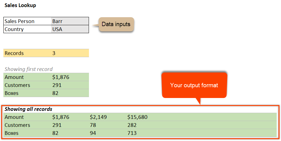
7. Multiple criteria (multi-condition) Lookups: In this video, we are going
to learn how to build a multiple criteria
look up using Excel. Specifically, we will
create something like this wherein you can input a
salesperson and a country name, and then you will
get these results. Let's do a quick
demonstration here. I'm going to change this to chess and leave
the country as UK, and you can see that
the formula that I have written have calculated
that there are two records, and it is displaying
the very first one, which is also highlighted here. So how do we do a multiple
condition based lookup. Already know that if I
use Xp or something. So for example, X up
and then say chess on the name column of my sales table and
then get the amount, I will get the very
first amount for chess. So it won't be necessarily
in the UK amount. I mean, in this
case, it would be UK because that's the
very first value. But it could be something else depending on how
your data is adjusted. So for example, if we
change this to bar, then we want the bars UK amount, which is 2499, but
my X L formula will give me bars USA amount because that's the
very first value. So how do we do
multiple conditions? Well, the technique is
to use the concept of derived columns which
have covered in the previous video,
and extend that. For example, we will say
X look, look up for one, and then the lookup array
needs to be open bracket. Name column is equal to my
name, which is an L six. Multiply that with country
column is equal to my country. Then the returning
column should be o because that's what
we want to look up. Now, when you presenter, you will get the correct result, which would be 2499. But how does this work? Okay. Well, let's go and
understand this. Here we are saying look up one, and then we are taking a list, which is my sales name column, and then checking
that against L six. If I just do this bit, and then evaluate that to
evaluate a portion of formula, you can select that
and press control equal to or the F nine key, and you will get the
evaluation results. It would be true wherever
the person is bar. So you can see that
the second value is true because we're
checking against bar, and then the fifth value is also true because the
fifth person is bar. This same way, this list will also be a bunch of
true and false values. When you take a bunch of
true false values here, multiply them with the
true false values there. Wherever the corresponding
values are true in both lists. That means name is
equal to bar is true. Country is equal to
UK is also true. The net result will
be two times true, which will be one
in Excel world. Because Excel treats
true and falls as zero, one and zero, so one
times one becomes one. That's why we're
looking up for one. We're saying look up for one and then do all of this
multiplication here, and then get the amount. Wherever that is one, it will produce a list of ones and
zeros, this entire thing. If I select all of this and
press control equal to, you can see that
this is actually zero all the way through
except for the fifth record, which is bar and UK. The next look up will say, I found the matching item
at the fifth position, so it'll get the
corresponding amount from the amount column, which would be my 2499. This is how I have
written that formula. Only additional bit
that I have done is I've put in information, no info message whenever
there is nothing found. Then I did the same for
customers and boxes. When we put this, it'll
give me that result. Now let's try bar USA wherein we have multiple
records. We have three records. Because XL will only
find the very first one, I'm showing an optional
message here and printing the very first
record details alone. Am I calculating the
number of records? Well, this is very simple. We can use the countifs
function to search for how many times bar and
USA combination appeared. We'll say name is bar, country is USA and then
they'll give me three times. Here I'm saying if my number of records
is greater than one, then just print the
message showing first record, else keep quiet. This is how that is constructed. You can take this
particular technique and extend it to any
number of situations. Now here is one extra
project for you? You can treat this
as class project. How would you fetch all
three records and show them? Instead of one, I want you to show number two and number three underneath using the
other techniques that we have covered in
the previous videos. Treat that as a challenge, and then if you are
having some trouble, check back the solution workbook in the
description links. See you again in the
next video. Bye bye.
8. Making nested IFs go away with LOOKUP() function: In this lesson, I'm going
to demonstrate how to calculate bonus using
the lookup formula. Here I have our employee data, and we would like to offer
bonus basing on these rules. Salary up to $60,000, you will get 5%
bonus up to 75, 4%. And if your salary
is up to 90,000, you get 3% anything
above, you get 2%. So how do we
calculate the bonus? You might be tempted to
write a long nested formula. But you can use a shorter
lookup function to do this. Before we do that,
we need to actually set up our bonus data
in a table format. You want to adjust your data in such a way that the
fast item is zero, and it would tell you what
is the bonus for that. The way to read this is zero
to 60,000, you get that. 60 to 75, you get this, 75 90, you get that. Anything above 90, you get this. That's how you want to adjust your data and create
a mapping table. Once that is there, you can use the lookup
function like this. Look up, Notice that
this is not up, H lookup, or x lookup, it is a simple lookup function, and select the salary, and then look up vector is the first column
of your table, and then result is the
second column of this table. Now, if this data is
not in a table format, it is in sell ranges. Make sure that you are
making all of these as absolute references by changing them into the dollar format. You can select the entire
range and press F four, and EXL will add the
necessary dollars for you. Once this is done, close
the bracket, hit enter, and EXL will calculate the necessary bonus percentages and print them there.
Let's double check. This person is getting
75,000 salary, they should be on 3% because they are above 75,000
not up to 75,000, so they'll fall
into that bucket. Whereas this person is
making more than 90,000, so they'll go into 2%. That person is under 60,000, so they get 5% like that. This is how I can calculate
my bonus percent. I can also calculate my bonus dollar amount either by taking
this and multiplying like this or changing
this formula and taking the lookup result multiplying with that
rate salary value. Go ahead and use lookup function instead
of nested formulas. Only thing of caution that
you need to keep in mind is this table need to be
sorted in ascending order. You can't really put
them in out of order. You need to go from zero
and set the boundaries clearly so that the values can be featured
correctly by Excel. I'll see you again
in the next video.
9. One Lookup and Multiple columns as result: In this video, I'm
going to show you how to use both x loop and up to fetch multiple columns
with a single function. So for this purpose, we will put our search name into
the J four cell, and we will instantly
see all the details of that employee either
horizontally or vertically. So let's understand this. I'm just going to type
chess bottle here, and instantly, I will
get all the results. Now, this is not
actually five formulas. This is a single formula. So how does it work?
Let's start from scratch. We say x lookup value, and then where is the look up
item, so it's in the name. But when it comes
to return array, instead of selecting
a single column, we will select the entire table and then close the bracket. Notice that the return column is not restricted
to a single column, it will give the entire
row of chess bonel here, and then it'll print it
nicely along the screen. This is a functionality
that is introduced in EXL 3605 along with the
L cup functionality. So every time you
write the clo cup and provide more than one column
as a output criteria, it will automatically take the values and spread
them on the screen. This behavior is
called spell behavior, and this whole functionality is called dynamic array
functionality. We have seen this elsewhere in the filter formula
example as well. While this is good, how do I take that and
turn it vertical? Well, you can use
that along with the transpose function.
Here I'm doing that. Again, I'll show
it from scratch. We'll say x, chest bonnle
in the name column. Let's not get the whole table. Instead, let's get just
the gender through salary. This is the return column, and we will get four results
going across the screen. Now instead of going
across the screen, we can then use the transpose
function at the beginning of this and send the cup results to the
transpose function. What transpose does is, it will take a bunch of values and change
the orientation. If you send it a bunch of rows, it will turn them into
columns, vice versa. Here transpose takes that and it will flip them and then show
them across the screen. Now, let's see this applied
for a different format data. Here, I got my names, and then every
month, sales values are listed in a matrix format. And I want to know
for a given name, what is the Q q total. Q q here would be October,
November, December. Here is my XL cup formula. Sum of Andrea Kimpton cup of a Kimpton in the name column, and then we want the results to come from October to
December columns. And then once the cup
gives those three values, we just sum them up. You can also use this with
the good old loop like this. You would say sum of lookup Andrea Kimpton
on the sales table, and the returning should be 11, 12 and 13 columns
within curly brackets. And then you'll say false. What loop will do in this
situation is it will return all the three
values as a list, and then sum will sum it up. Now, if you're using this
function within Excel 365, you can just press enter. But in an older
version of Excel, you can still use
this construct, but you must press control, shift, enter to get the result. I'll see you again
in the next video.
10. Combine two tables (consolidation) with Lookups: In this lesson, we
will understand how to combine two tables using
the lookup formula. Here I have slightly
longer employee dataset with 1,000 employees, and we have several columns
of employee information. But we also have another
part of the puzzle here with their name and date of birth available in
a separate table, and we would like to merge these two to create one combined view. So here, for example, I can say date of birth, and then use either
up or x lookup. So we'll say X, my
lookup value is name, and then the lookup array
is the name column on the DOBStable and the return column
is my DOBS date of birth. And when you close this,
you will get some values, some places where the
employee doesn't have a corresponding date of
birth, you will get an error. Let's just fix the error
first so we can go and then either blank it out or put something else like
date of birth missing, and then select
this entire column, quickly apply a
date format on it, and we will have our date of
birth information available. So this is how you can use the Vp or X lookup to
combine two tables. Now, let's make it a
little more complicated. What if your date of birth
table doesn't have the name, but it has last name
and first name as two separate columns and
the date of birth value. Here is how you can do this. Add a new column. Let's call this DO two. In this column, we will write
a look up formula so that we can take the full
name here and match it against the combination of last name and first name there. Let's make a note of
this stable name. Stable is called DOB S two. We can write the formula
here directly now X Loop value is my name. Look up array needs to
be the combination of fast name and last name
columns of my DOBS two table. This would be DOB, fname, ampersend space, and then
ampersen DOBS two last name. Notice how with the
Luka para itself, we are taking two
different columns of that table and
combining them, and then return
column needs to be DOBS two date of birth. Then if there is no value found, we will just print a blank value and we will again
get the result. Let's apply some formatting. You can apply date
formatting from home here, but here is a shortcut that
I normally like to use. I like to use Control
shift three to quickly turn values into date
format with DMM y format. The idea of using two columns
and combining them here is similar to the idea of derived columns that you have
seen in some other video. Both these approaches give
you a powerful way to combine data even if the
formatting is not consistent. I hope you found this helpful. I'll see you again
in another video.
11. Extract data with lookups from a Big big table: In this lesson, I'm going
to show you how to extract a few columns and rows
from a large dataset. So here I got 1,000
employees data, and we have several
columns of information, so it goes all the
way up to column CD. And this is all
randomly made up, but this kind of datasets
are quite common. In fact, I had to use
a similar technique at a client's place several times throughout last year.
So how do we do this? Let me first explain
what's going on here. I can select any
number of columns. I can specify them here, the column numbers that
I want to extract, and then I can give the names, and this part here will
show me the relevant data. So for example here, instead of two, I want
the column number three, I put three there,
and instantly, I'll get job title, and then
the title gets printed here. I can change these order. They don't have to be like this. So for example, after
three, I can have two, and then seven, and then one, and I'll get the
details as shown there. So how do we do this? First up, set up your original
data in a table. It doesn't have
to be in a table, but having it in a table
makes your life simple. So in our case, I put this
in the table named staff. And now we go to
the extract page. This is where we would
like to extract. The bare minimum you need is the names or the
unique identifier. So in this case, I have my
names listed in column C. And then I also need to identify which columns do I want
to extract in what order? So print them on the screen
along the way like this. And now for the first row, we will use the index formula to get the second column header, seventh column header,
sixth column header, and print them there. This index formula
goes like this index of my staff table hash headers, So this will give you access to all the header information
on the staff table. And then the header that I
want here is number two, so we'll point to that
and close the bracket. I'll get the header for the second column,
which is gender, and then we just drag this sideways to see the relevant
headers for everything. Now comes the bit where
we have to extract this. I'll just delete this and
we will write the formula. So we want to do an X look on this value in the
very name column. So we'll say staff name. But what do we return. Now, the column that we
need to return would be two here because
that's the gender column, but it would be seven here, six there, 12 there. So the column that
we want is dynamic. This is where the index
function comes in handy. We'll say index of
the staff table. We want all the rows,
so we'll just say a to indicate that I don't
want a specific row, I want all the rows. But the column number that
I want needs to be that, so we'll point it to D four. Now, you need to make some of these references
mixed references. This will always be in
the row number four. I'm just going to change
this to D dollar four. Likewise, this needs to
be always in column C, so I'll change this
reference to dollar C seven. Again, to change these
reference styles, you place your cursor
there and keep pressing the f four key until you get
it into the desired style. Once this is done, we
close the index formula there and then close
the bracket. That's it. We'll get the gender
Copy this formula, select this entire
range, control, and you will get the results here in a nice,
beautiful manner. This is all dynamic. In fact, when I built
something like this, one of my colleagues at a
client's place saw this, and he was super impressed
that he took a copy of this, made a blank spreadsheet
template so that he could use it to make payroll extracts every
time he needs that. So I hope you found
this technique useful. Now, you don't have
to use X Loup. You can also use hep to do this. I'm not explaining
this part here because we've already covered hop
and lookup at length, but feel free to take it up
as a challenge and write the Vp basic formula or refer to the download file
to learn how to do that. I hope you found
this lesson useful. See you again in the
next one. Bye bye.
12. 8 Common lookup errors & remedies for them: In this lesson,
I'm going to talk about eight looker
errors in the fixes. These errors are
value missing error, value not really missing
error, incorrect answer, typo error, data error, reference error, column error, and then formula won't work. Let's go and see what these are. The value missing
error is by far the most common error that you see when you're using
the lookup formula. So for example, if I'm
using either x lookup or v lookup and try to look up for something that is not there. So in this case, I'm
looking for Chandu in my staff name column
and try to get the salary of Chandu
I will get hash A, which is the common error that you see when the
value is missing. So how to fix this error. Within xp, you can use the
not found option to fix this. For example, I can say not found here and that'll print
the message not found. Within Vp, same formula
becomes something like this. So we look up Chando
staff five falls, and this will be an error, and we can use the if error
function to prevent this. When the help has an if error, that means it is an error, then not our employee
will be the message, and it will print that message. For the next type of error, imagine we have a value
of chess bonel here, and I want to really
look for this person. So we will use we look up. We'll look up the name
in the staff table, and then they get
their gender false. Now, we could see that
clearly chess bonel is there, but we get error. This is kind of like
value, not really missing. This is because we think
this is chess bonel. But when you go
and edit the cell, you notice that
there is actually an extra space in the end, which is throwing that
problem. So how to fix this? Well, the number one fix
is to remove the space, so we can go and delete this
and that'll fix the problem. But if you cannot edit
this for whatever reason, the other option is to use
a function like trim on your input data sets so that you can remove any unwanted spaces and get the correct result. This will work with Luka or x. The third type of error
is incorrect answer. Here you can see
that I'm looking up chest bonel but I'm getting
their gender as female. Whereas here in the table, their gender says male.
So what's going on? This is because when you
use the lookup formula, if you forgot the last
parameter and leave it out, Excel will default that to true, which means it is going to
look for an approximate match. This means it will
go from the top. It will assume that your list is sorted in alphabetical order, so it's going to look
for chess bonel. First person is B, second
person is D. Excel assumes that because B and then C is no longer
there and it is D now, I'll give you the answer for B, which is female here. To fix this, you need to specify the last
parameter as false. Another alternative is to
use x lookup wherein you don't even have to specify
the type of lookup mode. It will always be
an exact lookup. That will also give you
the correct answer. Here is our next
error type error. Whenever you make a
typo in your formula, you're more likely to
get the hash name error. So when you see the
hash name error, it means you've made some
sort of a typing mistake. Here I got my Xp formula. Everything looks all right, but on a closer inspection, you can see that we misspelled
the X lookup as x LUK. The moment you fix this, it will sort that problem. Another common type of
typo that people make is give a wrong
name in the table. Either table or
the column itself, if you misspell, you'll
get the type error. Now these type of
typos are easy to catch because the moment
you try to presenter, Excel will give a
warning message saying you're trying to type something that
doesn't make sense. That is when it will
also highlight that this part of the formula
is not meaningful. This is very easy to catch. But the other type
of typo errors here, they're not easy to catch and XL will throw the
hash name error. The next type of
error that you would make is a data error. Let's say got an employee
name like Douty Strutle here, and we want to see
their department. So I say X L this person on staff name and then
staff department. And then we get hash value
error. What's going on here? This is because when
you observe your data, you notice that their
department value is indeed actually hash value. This could happen
quite commonly when you try to copy data from another system or
another spreadsheet, and if there was an error
in one of the calculations, then that will kind of
percolate and show here. Now, this kind of an
error is hard to trap. If I put, for example, staff department and then if
not found as value error. This won't still show. It will give you the hash value instead of that
specific error message. This is because technically, we did find the Doughty Strutle, it so happens that their data
itself is giving an error. This is where you
could either use the error function or you want to inspect the data quality and fix any errors there. The text type of error
is a reference error. This is when you try to refer in your formula to something
that no longer exists. Let's do this with a
simple formula here. We will look up for
Doughty Strutle salary. Staff name and
then staff salary. We do get the answer here. But the moment I go and
delete this column, I will get a hash error here because I no longer have access to that
particular column, so I'll get the hash rah error. This type of error
is quite common, especially if you
refer to things in another spreadsheet
and you close that file or things like that. When you get the
hash wrap error, you need to go back and check if your formulas have things
they need to work. Seventh error is a column error, and this is very, very
common with p formulas. So let's write a look up here. We got Dotty Strutle
and then we'll say up Dotty Strutle
in the staff table, and then we want
their salary column, which is five on falls. And we get the
correct result here. Dotty salary is 41,980, and that's what we
are getting here. But notice what happens if I insert a column in the middle. It doesn't have to be right in between salary, but
it can be anywhere. As long as salary is no
longer column number five, it is now column number six, this value becomes
zero because this up has no idea of what just
happened on the screen. It is still happily referring to column number five instead
of moving that to six. So when you make
these kind of things, this will be a colmeror again, this is very hard to
spot because there is no visual indication
of what happened, and it can be quite problematic, especially when you're working
in a team setting where other people are adding columns
or moving things around. This is again, another reason why you should use
XL cup functions. I will undo the steps and show you what
happens with X Lup. X, my value staff name, staff salary, and we'll get the same
answer here and there. But if I insert a column,
this one becomes zero, but this one still gives you
the correct answer because this is still technically referring to the
staff salary column, and it will work as long as nobody went and
renamed the column. This last one is formula
won't even work. This is a very tricky
one. I'm going to write the formula and then you'll
see that it won't work. If I say X and then we'll
look up this value. Staff name, staff salary. Presenter, nothing
happens, the formula remains as it is as if
it is a text value. This is because here in
this particular cell, the formatting has been
set to text format. Now, normally, el cell
formating would be either general or number
or date or currency. But this cell, I have
already set it to text. Either you might do this
accidentally or somebody else might have done it
for some other purpose. But when you have a cell
as text formatting, any formula you type in
that cell will not work. Easy fix, change the
formating back to general, and then edit the
cell and press enter, and now the formula will work. So there you go,
eight lookup errors and easy fixes for them. I hope you found this lesson
in this entire course very useful for leveling up
your loop and X L up game. Thank you so much for watching, and I'll catch you
again somewhere else.
 Chandoo, Become Awesome in your Work