Learn Excel for Data Entry: A Beginner’s Guide!

1. Welcome & Course Introduction: Hello there. I want to start by welcoming you to this course. My name is Sadik Umer, and I'm going to be your coach throughout this course. This course is designed for complete beginnss. This is an Excel course for data entry, and it is going to be complete beginners. Even if you have never used Microsoft Excel in your life, you will be able to follow along, and by the end of this course, you will have the right skills and the capability to start performing data entry tasks with Microsoft Excel. I'm going to share all the basics from creating sheet, updating sheet, saving you a sheet. What is even ros? What is column after using some basic formulas that are going to help you clean up and organize your data. And this course is going to be very helpful for you if you want to maybe become a virtual assistant and you want to start opening data entry as a service to client or even just a freelancer, operating data entry service to client. And it is also going to be very helpful to you if you just want to add it as a skill in SCV. If you want to maybe get hired as an administrative assistant or an Opie assistant, Microsoft Excel is something that you are going to want to be using because data entry is a task that most administrative assistant and office assistant use. At the end of this course, I'm going to show you a real world example of a data entry task. I'm going to share my scorer and show you a real simple work, a real work that I did for a client. Going to show you how I did the work so that you'll be looking over my shoulder and you'll be able also to practice polo along, and you can even use it as your work sample. So if you are ready to get started, learn Excel from A to Z and start using it for data entry. This course is absolutely for you. I have been teaching data entry on YouTube for a few years now, and I decided to make this course because data entry is a service that is in constant demand. It is very helpful for anyone who wants to start virtual assistance or even if you want to just work in the administrative support industry, you need to learn it. Microsoft Excel is a big part of data entry, and that is where I specifically made this course. So if you are ready to master Excel and start performing data entry task, I'm going to see you in the next lesson of this course. Thank you for being here. 2. What is Data Entry? (VA context): So in this lesson, we are going to understand what exactly is data entry. Data entry is simply the process of updating some data, inserting some data in an easy way for people to read and understand. A good example is I can send you a Microsoft Excel pile or I can send you a CBS pile with a lot of data. Maybe I can go to a property listing website like Zero and export a list of data with maybe 1,000 list of properties in the data, and I can send it to you and I will say, I need you to get me all the properties that their price is $300-500 thousand. And the properties has to be in a certain area. And I want the data to be in an easy way for me to understand which property is in that area and which property is in that area. The data is messy. There are a lot of random data in the file, maybe 1,000 rows of data in Microsoft Excel. And your job is going to be to sit down, take a look at the data. Clean it up, delete all the properties that are not relevant, all the properties that does not meet the client criteria, you delete them out from the spreadsheet, and you make sure you leave only the ones that meet the certain criteria, and you expand the row and the columns, make sure everything is good and easy to read and understand so that at first look when someone look at the data, going to be able to read everything in the data and comprehend. This is an example of data entering. 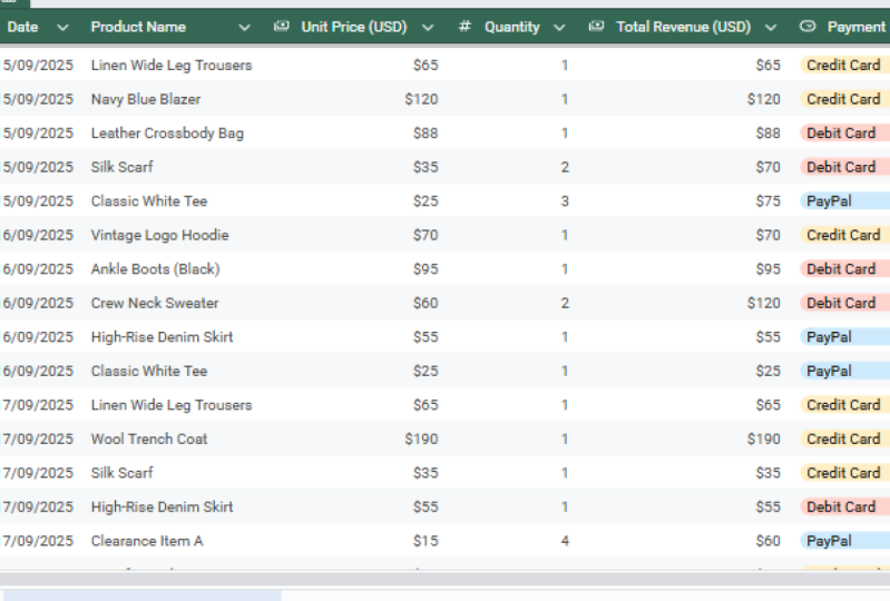A client can also send you a PD file with some pon numbers, random phone numbers, and people's names and addresses, and your job will be to go through the document and find people who live in a certain area and you list them out with their contact information. And another example is someone who have an e commerce website. If they have maybe 1,000 product listed on their website and they have all the product in a spread sheet. Your job will be every day at the end of the day, you go to the spot sheet and you compare the quantity of each product that they have in their store, and you compare it with a number of products that they have in a spread sheet, you make sure you update Everything so that it correspond. One look, they can take a look at the spreadsheet and see each product with the number of quantity of each product that they have and the availability of the product. This is another example. Data entry is simply the process of getting some data random data that is hard to read and hard to understand and you organize it, make it easier to look at, easier to understand and easier to read. This is a general explanation of what data entry is. And in the next lesson and the follow up lessons, we are going to see examples real examples, and we are going to actually get to doing the tin, so that you'll have even a better and clearer understanding of what data entry is. And in the next lesson, we are going to look at the different types of data entry services that virtual assistant offer so that you'll have even a better understanding of what data entry is and how to use Excel P data entry. I will see you in the next lesson. 3. Types of data entry tasks VAs do: So in this lesson, we are going to understand the type of task, the type of data entry task that virtual assistant do. And the first thing we are going to look at is the basic data entry task. The basic data entry tasks include copying data from one pomat to another. A client can send you a PDF file with some data in it, and your job will be maybe to copy the data from the PDF and type it out in maybe a microsoft word. Or Google Doc, and the client can send you a screenshot or they can maybe even snuff a piece of paper with some data in it, and they will send it to you and you can just copy the data and put it in a Microsoft Excel pile. A good example is I previously worked for a client who is working with client herself. And when she is having a call client, she is a therapist. So when she is having a call with client, she is taking some note, some random note. When she finished working with a client, she will take a snap. She will snap her note. A piece of paper, and she will send it to me. And I'm going to organize it in a Google Doc. I type it out with the name of her client, and I put all the information so that whenever she just want to take a look at the client information, when she open the Google Doc, she see the name of all the client. If she open each name any client, she is going to see all her notes that she type out in a piece of paper. So this is one example of a data and Teddy tax, which is under the basic. Other example of a basic data entry task is copying and fsting data from one document to another. Let me give you another example. If you are working for a real estate in Besto, they can send you a Microsoft Excel pile with maybe 1,000 list of properties. The properties have all their addresses all across the US maybe, and the properties are around different ranges, and maybe there are mobile homes in it. So different types of houses. There are single family homes. There are multi family homes. The apartment is one big list with a lot of data in it, and your job might be to categorize it to make it easier for the client to see properties within a price range within one price range, to see each properties in each dipendent state. So your job might be to create maybe it is one pile, you can create ten dependent Google sheet. You just go through the big list and you copy each property that is located in each different state, and you put it in a different separate sheet, and you pick each property that is within maybe a price range and you paste it in another separate sheet. You are copying data from one pile and fsting it to another pile to make it more organized and more easy to read and understand. An example of a data entry tax that is a little more advanced than the basic copy and fest type is maybe doing some data validation. An example is a client can send you a pile a lot with a lot of data in it, and your job might be to maybe calculate all the average prices of each home. Maybe the houses are maybe 1,000 houses, 1,000 properties on a spreadsheet. And the client want to know the average price home in maybe California. So your job will be to pin all the properties that are in California and you put them in one spreadsheet and you use a pomula to pin the average the average price of the houses in California. So this is a little more advanced. You are going to have to use some pomelas and data validation and some Pless in order to figure it out. Other example is collecting some data from contact pom and organizing it in a Google separate sheet or in a Microsoft Excel. One example is maybe a client has a pom on their website that people are going to pull out a pom and submit for whatever reason, or to make it even simple, let's say you are working for someone who is a recruiter. Recruiting for other people. And maybe every week, they are posting a job application and 1,000 people are applying for each job. So your job will be after the application close, you go to the back end of the form and you download all the people's responses, maybe in a CBS pile and you go through the responses, the client is going to give you the criteria to go through. If you are looking, you go through all the people who submit the application. Anyone who didn't provide this kind of information, you delete them from the list. Anyone who didn't meet the criteria, you remove them from the after you finish removing all the people that doesn't meet the minimum requirement, then you clean it up, arrange it in a way that it is going to be easier for your client to go to the responses, and you send it to the client. So these are just some type of data entry task that you are going to be doing using Microsoft Excel. In the next lesson we are going to look at, why do client even hire virtual data entry virtual assistant? Why is data entry important? And why do client hire someone to do data entry work for them? Because clearly data entry work is not very hard. Microsoft Excel is not very hard to learn. Most clients who are going to hire you to do data enter work for them, they know how to use Excel themselves. So why will they hire you? That is what we are going to look at in the next lesson. So I'm going to see you there. 4. Why clients outsource data entry: So why do client outsource data entry tasks to virtual assistant? Since clearly data entry using Microsoft Excel is not very hard. Almost anyone can learn Excel in a short amount of time and do data entry work. So why do client for a part to hire someone to do it for them? And I can tell you the one single reason why. Most times most data entry task is time consuming. It takes a lot of time to do data entry work, most of the time, and that is a key reason why client hire virtual assistant and outsource data entry task. That is why it is a good thing for you, virtual assistant because you don't have to be an expert in specific things before you get hired. Client just want you to save them time and if you can save them time, they can give it to you. That is why the first step is just learn how to use Microsoft Excel. If you learn how to use Microsoft Excel, good NOP, then you just learn how to present yourself and you will be able to find client without being an expert in anything. Because client outsource data entry tags. Because it is time consuming. Even if maybe I have employees who are working for me, the employees have the parental responsibilities. So sometimes it is going to be challenging to pass on data entry tax to someone who is maybe an administrative assistant. It's hard maybe to pass on the tax to someone who is currently handling other things, and that is why client for the part to outsource data entry service to virtual assistant. And it's very rare to find a company hire a data entry employee. Companies hire administrative assistant and personal assistant administrative officers, things like that. But data entry, most times a client, if someone just won't get data entry tax done, we hire virtual assistant because it is easy to do. Even if you don't know how to do it, it's easy to learn Microsoft Excel after you learn Microsoft Excel. You can start performing data entry tax without too much trouble. And so in most cases, it's easier, it's cheaper to hire someone to hire a virtual assistant to do data entry work for client instead of them doing it themselves, or they pass it on to someone on their team to take care of it. And this is the end of this module. And in the next model, we are going to actually get started in the tutorials. I'm going to show you how to start even navigating how to access Google Sheet and Microsoft Excel, how to navigate how it works, the rows and columns, how everything is in Microsoft Excel and Google Sheet and how to save your work. So I'm going to see you there. 5. How to access Microsoft Excel (Web/Desktop): This lesson, I'm going to share my screen and show you exactly how to access Microsoft Excel and also how to access Google Sheet. But before we do that, I'm going to explain to you the differences. Microsoft Excel is a software that you install in your computer. It's a software that you install the same way you install a browser, a Chrome browser, a pre Box, is an a, a software that you install in your computer. So you have to have it in your computer and do your work on your computer. When you use Microsoft Excel, you can only use it on your own. When you finish, you save your work, you save your work on your computer. If you open another computer, you cannot access that pile that you work on on your computer. If that Microsoft Excel is only on your computer. This is one major difference. The Google Sheet. Work the same way. You can do almost anything that you can do in Microsoft Excel, you can do with Google Sheet. But the difference is Google Sheet is online. You use Google Sheet, you just log into your browser, open your browser and log into Google Sheet, and you can just open and start working with it. And if you start working in Google Sheet, you can just close the browser. If you open another computer, you can simply log into your Gmail account and you will have access to that same Google Sheet. You can share the link with anyone online, and anyone can access you a Google Sheet and you can even collaborate and work together. So in most cases, it's easier to use Google Sheet because it is online, it is free, and you can do almost anything that you can do with one, you can do with the other one. Okay, so I'm going to share my secret now and show you how you can access Microsoft Excel on your computer. And how you can access Google Sheet online. So the first thing I'm going to start with, I'm going to show you how to access Microsoft Excel on your computer. And what you just need to do is if you open your computer, you just click Windows or Command. If you click on Windows, you can see Micro, you can see Excel here. But if you didn't see Excel, you can simply search it in the search bar. Right here, when you search for Excel, you are going to Cesar up. This is it right here. You can simply click on Open in order to open it. This is interface of Microsoft Excel on your computer. You see this new when you click New, you are going to create a new Microsoft Excel pile. Or you can simply click here Blank Document. These are some welcome to Excel pile and a Poma tutorial. These are all things you can explore. And if you click here, you can see more template. But if you just want to start working with Excel, you click on this blank workbook and a blank workbook is going to offen. This is your blank workbook that you can start working on. You can start working on your blank workbook and start saving your files. So this is how you can access Microsoft Excel on your computer. Next, I'm going to show you how you can access Google Sheet online Google Sheet. And in order to access Google Sheet, we have to go to a browser first. The first thing you need to do is when you open your browser, make sure you are log into a Gmail account. When you are logged into a Gmail account, then you can simply go to the searchbar and go to docs dotggle.com. Do dotggle.com. Okay, when it finished loading, this is Google Docs, and we are not going to work with Google Docs. We are going to work with Google Sheet. So you need to come right here to this menu icon. When you click on it, these are all the Google tools you can use. But in this today we are going to use Google Sheet, so you click on Sheet, and it is going to take you to Google Sheet. And alternatively, you can just go to docs dotggle.com slash CEPEDSHeT. If you go to this link, you are going to land directly on this page without even using the Menu icon. So when you are logged in, if you have created other spreadsheet, you are going to see them here. But if you have no other Google Sheet, this is going to be empty. In my case, this is empty. I have never created any Google Sheet with this GML account. If you want to create a new Google Sheet document, you will click on this big plus icon. If you want to take a look at some template, these are some template you can take a look at. If you click on this template gallery, you can open some template and just go through them and see if there is anyone that is close to what you want, so you can start working with it. But if you want to start with a blank document, you click on here, and a blank document is going to offen. Okay, so this is Google Sheet interface. This is just some sidebar that you can use to add tables, but we can collect this icon to close it. And when we close it, this is our Google Sheet pile. You see it looks a lot like the Microsoft Excel one. See the differences is just in the menu. Different things are located in different places, but in terms of the interface is almost exactly the same. So this is how you can access Microsoft Excel and Google Sheet. Throughout this course, I'm going to be using Google Sheet because it is just more accessible and easier to use. And if you want to practice in both places, then you can simply practice in both places. So I hope right now you understand how to access Google Sheet and Microsoft Excel. The next lesson, I'm going to show you how to navigate Google Sheet, how to navigate the sheet, how to navigate the menu items and the rows and columns. That is what you are going to talk about in the next lesson. So I'm going to see you there. 6. Navigating the Excel interface: This lesson, we are going to go over the interface of Microsoft Excel. I'm going to show you how to navigate the interface. We are going to be using Google Sheet. I'm going to show you how to access all the menu items and how to access all the rows and columns. That is what we are going to look at. So I'm going to share my skill so we can get started. So after you log in you create a new document, this is what we are going to look at a blank document. And the first thing I want to show you is this navigation menu right here. This is where you are going to navigate and do almost anything that you want to do. You see, when you click on Pile right here, you can create open a new spreadsheet, create a new one. If you have a Google, if you have another separadset on your computer or if you have a Microsoft Excel pile on your computer, you can click often and find it in your computer and upload it. You can import it. These two items do the same thing. You can make a copy of this current spreadsheet. You can share it with other people. You can download it. You can change its name. We are going to go over this more details later in the course. And if you click on Edit, you are going to see Undo and Redo. If you do something you make some changes and you want to undo it, you click here or you click Redo and you can see a shortcut. The Undo, you can click here or you can click Control Z to undo or click Control Y to redo. You can cut, copy First and First special. This we are going to look at them later in the course. But this navigation menu is where we are going to be making a lot of changes. And these other items right here, this is where we are going to make pomatin changes. We are going to use these items, these little icons. We are going to use them to pomat all the data that we added in our spreadsheet. So this is where you will write all your data, add all your data, and this menu icons. This is where you are going to pomat your data, make items bold, italic, add colors. This is where you are going to do everything. And this navigation one up here, this is where you are going to make changes that affect the entire separate sheet. And you see sheet right here, this is the sheet we are working with. If you collect this plus icon, you are going to add another sheet and you can add different items here. And when you come here, you see a separate is a dperent separate sheet. So in case a client share a big pile with you, you can see a pile with diperent sheet, and each sheet is going to have its own data in it. So this is just a general basic of the interface and how the interface works. In the next lesson, we are going to understand in more details what is a cell what is a row? What is a column, and what is a sheet? I'm going to see you there. 7. Understanding rows, columns, cells, and sheets: In this lesson, we are going to understand what is a cell, what is a row, what is a column, and what is a sheet in Excel. I'm going to share my scurnce so we can get started. So the first thing we are going to understand is what is a column. A column is simply the line under this alphabet. If you click on this B, for example, you see everything that is under this B is in column B. If you click on D, everything that is under D is in column D. If you click here, you see this thing that you selected is under column G. So everything under the alphabetical things is a column. And these numbers right here, this is what is called a row. When we click on three, everything that is in this line is in row three. If we click on this six, everything in this line is in row six. When we click on this, before we do this, what about the boxes individual boxes? This individual boxes is what is called a cell. This individual box, each one box is one cell. And this cell that I just selected, it is in column D, row eight. So it is in Deight and you can see it right here. The number the name of it, the name of this cell that I selected is Deight. If I choose this one, it is H ten. You see it is under column H and row ten. So this is what is column row and sell. The next thing is sheet, which is what we previously explained a little bit. This is sheet one. This is sheet two. You can have several sheet and you can have different data and diperent sheet. You can have one sheet with maybe a list of names that start with A, and you can have another sheet that has list of names that start with B. You can have one sheet with list of properties that are in California. You can have another sheet that has list of properties that are in Arkansas. So this is what a sheet is. So I hope now you understand what is a what is a column, what is a cell, and what is a sheet? The next thing I'm going to show you in the next lesson is saving you work. So I'm going to see you there. 8. Saving your work (local & cloud): In this lesson, I'm going to show you how to save your work. It's important to continuously save your work. When you start working with Excel, as soon as you make any significant change, it's important to save your work because for whatever reason, if you close a tub or if you close a pile, then you are going to lose all the work that you did. And that is why it's important to regularly save your work. And I'm going to share my screen so we can get started. So I'm going to start by showing you how to save your work online and also how to save your work. On your computer. The first thing we need to do before we even save the work, it is a Google Sheet, we can rename it. We can name our pile. You see right now it is said on a titled spreadsheet. We can simply click on it, click the backspace to delete everything, and we can write a name pull our pile. We can see something like some file, pull COs This is a name that anyone is going to see. Everyone is going to see when we share it with them. Oops, I typed it wrong. Okay? So when we share you a pile, this is how it is going to look like. And if you are working online, it is automatically saving all the changes you make. You see this cloud icon with a check mark, it means all your changes are saved. So when you make few changes, make sure you look at right here. If it is checked marked, it means your changes are saved. And if you want to access your work in any computer, when we come back here to all the spreadsheet that we have, if you on any computer with your Gmail account, you are going to find the pile right here. When you click on it, the pile is going to open and you are going to see all the changes that you made previously. This is how you are going to save your work in a Google Sheet. The next place is Microsoft Excel. In Microsoft Excel is a little bit dperent because it is on your computer. You have to save it on your computer. We can do that by clicking Control or Command S, and you just write a name for it. Sample pile, and you click here to choose a place where you want to save your pile. You choose document anywhere you want to save it, and you click on Sab. And that is it. The pile had been saved. You see the name that we add right here. And when you close it, if you go to the folder that you save it, you double click on it, you are going to open it and you are going to help all your changes exactly where you leave. In the next lesson, I'm going to show you how to start typing and editing content in a Microsoft Excel pile. So I'm going to see you there. 9. Typing and editing text and numbers: So in this lesson, I'm going to show you how to start typing and editing text and numbers in Excel. So I'm going to share my secret so we can get started. So right now I am in Google Sheet dashboard. You remember when you go to docggle.com slash spreadsheet, you are going to land on this page, and this is a sample pile that we previously created. In case if you didn't have this file, you can simply click on this big Button, this plus icon to create a new spreadsheet. But since we already have this one, I'm going to click on it in order to open it. Okay, now that our spreadsheet, often, I'm going to start by typhing numbers and text. If you want to start typhing anything, for example, if you have a PDF, if you have a PDF that you want to copy text from the PDF and add it in a spreadsheet, you can simply select each cell that you want the text or numbers to be, and you can start typing. But that is not all. Let me first show you this if I select this B, this column B, and I type maybe New Excel data. When I click on Enter, you see the I move to the cell below. If I go to if I use my arrows, my keyboard arrows, I can go to left, right off and down. And if I want to add numbers, I can simply type all the numbers that I want to type. But one thing you should note is, if you want to edit numbers or text or anything in Excel, not as editing in Google Doc or in note pad or something like that. Let me show you what I mean. If I want to maybe make changes to this text, I write new Excel data, and maybe I want to change it to new Excel data, Pomat, maybe something like that. You might think, since you already write new Excel data, you are just going to write Po Mat, since that is what we are missing, but that is not the case. If you select Zapile and if you write you just start writing Pomat you see the previous text that you write is over reading. It had been deleted, and now the new text is added. So how do we do that? If you want to add something to this content that you already write in this cell, instead of clicking on it and start writing, you have to come up here. This is called the pom lava. You have to come right here and you click on the exact position that you want to add the content. If you want to add the content at the end, then you add your so at the end, add space and write whatever you want. And if you want to add it here, you can add the so right here. When you finish writing all your content, you can click Enter, and now your content is added in this cell. Don't worry, you see the content is way over. You cannot see all of it because it's not enough. The length of the cell is not enough to accommodate all of it. You can easily drag like this. You click on this drag and often it to see everything, but we are going to go over that in more details. But this is the first thing that you shall understand. When writing in Excel text all numbers, you can copy data from any place if you have a PD, if you are typing data, you type your data, but if you want to make changes to the data that you already write, you cannot simply select the cell and start typing. If you do that, you are going to overrite what you already written. You will have to come up here to that pom lover and make all your changes. This is the first thing you shall understand about typing and editing texts and numbers in Excel. In the next lesson, I'm going to show you how to copy, first, cut, undo and redo. And I'm going to get some sample data so that we are going to have a pull data to practice so that you will have a better understanding of how it works. I'm going to see you in the next lesson. 10. Copy, cut, paste & undo/redo: In this lesson, I'm going to show you how to copy data from one pile to another without doing it manually. The way you can simply copy and fast, and I'm going to show you how to cut data, what it actually means to copy and fist and what it means to cut some data, and I'm going to show you how to redo and undo. So without any delay, I'm going to share my screen so we can get started. Okay, to get started, I'm going to delete this content that I practice with previously. And in order to delete, you can either click on the cell click Delete form your keyboard, select and click Delete. Or you can highlight like this and click Delete to delete everything that is inside. So now we have our empty sheet to start working with. I'm going to start by showing you how to copy and fast data, and I'm going to use Char GPT to get some sample data that I'm going to work with. So I'm simply going to go to chagpt.com. I'm going to use a prompt that will allow ChaGPT to give me the exact type of data that I want to start working with. 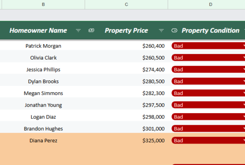And I'm going to use a prompt like this. So the prompt I used is I am practicing my Excel skills. Can you give me a sample data with columns for property address home owner name, property price, and property condition to practice with? I need PIPT loss or random data. Please forgot to say, please. So I'm just going to use this prompt and I'm going to see what JharPT is going to provide. Okay, great. So harGPTPvide the data, I can simply download it in an Excel Pile format, and I'm going to click Download. Okay, the pile had been downloaded. I'm just going to open it. When I click it, it is going to open in Microsoft Excel. Okay. This is the sample data that CharPT has provided. Throughout this course, I'm going to be using this sample data to practice and show you everything that you need. I'm going to click a level editing so that I will be able to copy the data. So I'm going to start by showing you how to copy and fist data. Let's say this is a pile that a client sent you. I'm just going to expand it a bit, or maybe I will not expand it for now, but you see this is a column for property address, home owner name. Property price, property condition. A client might send you this data. Maybe they export the data from a website like Zulu, and it has a property address, the home of the name of the home owner and the price and the condition of the property. Maybe they will ask you to fine properties within specific priceyrange, for example, they will ask you to pin properties that are within 300 and $400,000, and the property needs to be in either fair condition or good condition. So if that is the tax, you see this one, for example, you see the property price is $351,000. The condition is fair. So this is a good one to work with. So we can copy it and st it in our sheet that we are working with. So I'm simply going to click here click and drag. Click and Drag. This is all the data that I want to copy. I can click Control C. You see when you see this border, this moving border, it means you copied it. Then I'm going to come back to my Excel file to my Google spreadsheet. I'm going to come right here. Maybe I want to past the data right here. I will select this cell. I will click Control B to past the data. So you see now this exact data have been fested. We pest the data on this file. If I want to copy more, I will go through it. This one is too expensive. This one is within the price range, but the condition is poor, so we can go through. No, this one is too cheap. So you get the points. I am going to just try and find one that meets the criteria that I just mentioned. Okay, this one, you see the price is within 300 400,000 and the condition is good. So I'm going to copy this one also Control C. Then I come back to my Google Sheet pile. I select a cell below this one and Control B to fest it. And now we see we have this other property fested. So this is how you can copy pile from one sheet to another sheet. If you want to copy the header entirely, you can come back here. You select the header. You come up, This is a header, you select it all, Control C. You can come back here, select the top row Control B to paste it. So now we have the header with the property address home on name price and the condition. So this is how you copy data from one pile to another. The next thing I will show you is how to cut, how to cut data. Cutting data, it simply means deleting data, but you remove it from the place, but you have it in your keyboard. Let me show you an example. If I select this I select this entry. I write click and I do COD. And I come down here, I do Control B. You see, I remove the data from this line and I paste it down here. So COT it means you code it, you delete it entirely from where it is and you paste it in a different place where whereas if you copy the data, you paste it somewhere else, you are going to have the data in two different places. So this is what COD is. What about undo? Let's say you make this change by mistake and you didn't mean to do this. Maybe you meant to copy not cut. You can simply redo. You can redo in two different ways. You can come to edit right here and click Undo. If you click Undo, you are going to undo the change. You see, the data became right where it was. But the simpler way to do it is to use keyboard shortcut. Let me mode it back again. It is right here. If I want to use keyboard Shortcde, I can simply colic control, control, and that's it. I undo the change. So it's the same thing with using this or you use a keyboard shortcd, but using a keyboard shortcd make it a lot easier and faster. And what about If you maybe I do this. I pasted this right here, copy it again. I paste it right here. And then I undo. But I remember I want it back. I can simply redo by coming right here. Either click this button, or you can click Control Y. If you click Control Y, you see I redo what I undo. So that is what redo and undo means. And in the next lesson, I'm going to show you how to use pined and replace feature. Pine and replace feature is going to allow you to pine a specific data within a big, large number of data and you can make changes to it or you can replace some data. You are going to understand it more in the next lesson, so I'm going to see you there. 11. Using Find and Replace: So in this lesson, I'm going to show you how to use pint and replace feature in Excel. This feature is going to be very helpful if you are working with large file. Let me give you a good example. If maybe you export some data from a website like zio, since we use property as an example, you export a list of properties, a large number of properties, and you go through the data and you find out that the data has maybe the condition of the properties is either fair good, and you want to replace good with maybe poor, something like this. If you have a data, a big data that you want to change something across all the data and you don't want to go through 1,000 lines making the same changes, you can use pint and replace. And at once, you can pind all the data, all the specific items in the data and replace it without going through it entirely. I'm going to share my screen and show you so that you will have a better understanding. In order for you to have a better understanding, I'm going to copy more data and fist right here. Or simply, I'm just going to come to the next sheet, and I'm going to import this data right here, and I can the simplest way to do it is to just copy everything. I can colct Control A and to highlight and select everything and then Control C to select everything. Control A and Control C. Now I copied everything in this sheet, and I can come back here and I select the top cell and collect Control B to paste everything. So now I have all the data right here. And in order to use pin and replace, let me give you an example of this one. You see, among the property condition, we have poor need renovation, fair, excellent, and good. Let's say we want to replace poor anywhere that you said poor, we want to replace it with bad or maybe don't contact, or let's just say bad anywhere that poor I fear we want to replace it with, but so in order not to go through all the data and do it manually, we can simply come up here. To edit and we can come down here to pint and replace. When you select it, what do we want to pint, we want to pint for and what we want to replace it with. But All sheet. Much case, we can just leave everything as it is, and we can click Replace All. And we click on O, and we click on Done. So you see previously this is poor. Now it is bad, but you see anywhere that poor I fear, it is now replaced and it's bad. It is changed to bad. So this is how you can use find replaced feature to replace any item in your sheet without going through thousands of lines doing something very repetitive. The next lesson, I'm going to show you how to use some basic pomlas. I'm going to show you how to use some basic pomula to add off to have maybe an average number of properties or to have number of total value of each property on a spreadsheet, and generally how to use some basic pomula to make your work easier. So I'm going to see you in the next lesson. 12. Basic formulas: SUM, AVERAGE, COUNT: This lesson, I'm going to show you how to start using Excel pomuls to make your work easier and more efficient. Let's say you have a list of properties, a bunch of properties, just like the one that we have each one with different price range and we want to find the average price of a home in this specific category. How do you do that? Do you have to take a calculator and start doing it manually? No, that is where pomela comes in. You can use a pomula to add it all up and find the average. If you want to add up all the numbers, let's say we have 50 properties on this spread sheet, and we want to find the exact total val of all the houses on the spread sheet. We don't have to do it manually. You can use a pomula in order to find it. We can use account pomula. So there are many formulas that you can use to make your work easier. And more efficient. And I'm going to show you a simple way that we can get all the pomelas to do everything without having to even memorize every single pomula. So I'm going to share my screen so we can get started. So I'm going to start with the most basic one. Let's say we have these properties. Each of these numbers is the price of the house that we have in this room. So we want to add up all the prices and to find out what is the number of total value of all the houses on this spreadsheet. Simple way to do it is to use pom, sum pomular. And in order to use a pomular, you have to start typing equal sine. A pomula has to start with equal sine. When you type an equal sine, it means whatever you type here is going to be a pomular. So you see by default, we have Excel just gave us this formula. This is a pomula that we are going to use. It starts with S SUM, then we have a bracket, C two to C Pip one. What this mean is we want to count from C two to C 51. What is C two? Right here, EPs col. This cell is in C two. You see it is in column C and row two. So we want to add up from here all the way down to C 51. So we can either type it manually or you can simply click right here. And just like this, you have your total value of the houses. It had been added on for but you don't have to keep remembering pomulas. Right now, we have AI. And with AI, everything is a lot easier. What you just need to do is anytime you want to do any type of calculation, simply go to Char GPT. Tell Char GPT is the type of calculation you want to do, and Char GPT is going to help you with that. Let's say we want to find the average value of a house in this list. We are going to have to use a different pomula and I'm going to delete this one that we have by clicking delete. And I will simply come to Char GPT and ask harGPT for health. I will say, I want to pine an average number in Excel. What formula can I use? So you see the formula. Each formula has to start use an equal sign. And if we want to pin the average, we can just say equals average and we add a bracket and we type all the numbers. But this is not we don't have to type all the numbers, or you see the example, we want to pine from C two to C 51. So the formula is going to be equals average C two to C 51. And we can do that. We can come right here and we can type an equal sign, and we will type an average. And you see it right here, the pomula C two to C 51, and that is what we want. So I can click on it. And just like this, this is average number of a house on this list. And this is how you can find any type of pomula to use. Let's use one more. I will delete this. I can come down here. Let's use count account Pomula. And I can simply say, what about account formula? So what a count formula do is it count the number of cells that has numbers in them. You see, this is I think it already gave us an example, use the count function to count all numerical values. So right here, all of these are numerical values. So we can easily use this pomula to count all of them because they are all numerical values. But what if there are numbers? Some columns here are numbers, some are alphabet. Then if we use count, we are only going to count the number of cells that are in numbers. But if we want to count everything, if you want to count non empty cells, including text, every cell that is not empty won't count it, then we are going to use this formula. We are going to use this one to see how it works. We can say equals count A, and this is eight C two to C 51, and we have PPT cells. Remember, we already have PPT data, so we have 50 cells, and that is how you can use count pomula. So this is how you can use some average and count pomlos in Excel. And this is also how you can find any pomula count to do anything really to make you efficient previously, you have to memorize all these pomulas, but now you can simply a Char GPT, and CharPT is going to give you any pomula that you want to so up until this point, we are working with an ugly data. I am just showing you how it works, how to use all the functions. In the next model, we are going to start formatting the data and start making it look nice. So I'm going to see you there. 13. Formatting text (bold, underline, colors): So in this lesson, I'm going to show you how to start pomating your data, start making it look presentable and easier for people to see, read and understand. So I'm going to share my secret so we can get started. Okay, so this is our sample data that we are working with. And the first thing I'm going to show you is how to make something bold. Let's say this heading, for example, this is a heading, right? So we want it to be different than the rest of the content down here. So how can we do that? The first thing we need to do is we can make it bold so that it looks different. And if you want to pomat anything, no matter what you want to pomat just select it. Since you can select only one cell and make changes to it, or you can select multiple cells. In this case, we want to select the entire row, so I can simply click drag. So you see I select all of these cells. I select Po cells, and now I can make pomatin changes to all of these pour cells. API you want to make it bold. All you need to do is come up here. You see this B sign when you click on it. Now you see it is bold. If we remove the selection, you see this heading is bold, so it is now totally different than what we have down here. And if you want to make it maybe italic, just to separate it a little more, you can select it again. You can use this icon to make it italic. So you see it is now a little more different than the rest of the items. The next thing we might want to do is maybe we want to make the header have a different color than the rest of the items on this sheet. And we can select the header again, all the cells that are in this header, and we can come up here. We can use these two buttons to change the color of this header. If you use this palo color, this Bocket icon, you are going to change the background colour of these cells, whereas if you use this, you are going to change the actual color of the text. So we are going to start by changing the background colour. So we select this. We can choose any color that we want from these selections or we can collect this polos icon to add a custom color. So let's say I want to use maybe this red. So you see now the background color is red, but we want to make the text white since it doesn't look readable. So I can select this one. I can choose white. And now you see the background is red, but the text is white. So this is how you can change background colors and change the color of each text. And another thing we might want to do is maybe want to highlight each property that maybe need renovation. We can do that by highlighting it in a different color. And we can simply select maybe this one since it needs renovation and we can come to the color fill and we can choose maybe this light yellow. So you see at one look, we can highlight each property that needs renovation, and we can make it this light yellow. So at one look, you will be able to see any property that needs renovation. So this is how you can start formatting newdata, make items look bold, italic. Use color to make something more easy to read and more easy to understand. And the next lesson, I'm going to teach you all about alignment. So I'm going to see you there. 14. Adjusting column width & row height: This lesson, I'm going to teach you all about alignment. I'm going to show you how to adjust width and height of a column, a cell and a row, how to center everything, and generally how to make everything good in terms of alignment. So I'm going to share my security so we can get started. So the first thing I'm going to show you is aligning columns. Previously, our column when we copy and fest the data looks like this. You see property address not everything is visible, home owner name, not everything is visible. You have to click on it in order to view it. Or maybe let me just undo and show you right here. Let's say I type flow party address and details. So you see the text is property address and details. But since the cell is only this shot, we cannot see everything. Sum up eight is hidden. In order to see everything, we have to click on it and look at the pomola bar. That is not a very good way to work with Excel. So I'm going to delete this and assume this comes right here. So we have property addresses that are not totally visible and the header is not totally visible. There are two ways to adjust column width. The first way is to move your uso right here. You see the uso change when you hobble over this. You can double click right here. When you double click, it will automatically adjust so that everything is visible. This is one way to do it. The second way to do it is to do it manually. You can select right here, you hobble over it. Then you click and select and drag it's all the way to no matter how long you want it to be when you release. You see now we have property address column very wide. You can drag and reduce it a little if you want. So this is the first way that you can adjust this. You can also adjust all the columns all at once. You can click and select the first one and hold Shift and select the last one. So you see we select everything. And if you double click right here, in any one of those if you double click, all of them are going to adjust to pit everything that is in each column. And if you do this, if you select one and you drag it like this, all of them are going to adjust. If you do this, you see all of them are adjusting to the right size. So each column will be the same size if you do it this way and you can click and drag to reduce it. But this is often not a very good way to do it because you will align you will make it big depending on the type of content that is in each column. So I'm going to do it manually. I'm going to encourage this and maybe increase it a little more home owner name, I can increase it a little more. Property price, I can leave it like this. Property condition is also good like this. We can also increase the size of the row, not only a column. Let's say this is a header, we want it to be bigger than the rest of the Z rows. Can simply come right here, we hole over it. Right here, we click and drag. When we do this, you see now the header is a lot bigger than the rest of the cells. So this is how you can adjust width and height of columns and rows. The next thing is aligning text or aligning content in each cell. You see now that these columns are bigger, we have the text too small and way up. We don't want that. We want the text to be in the center. So we can click. We can highlight all the columns that we want to make changes to, and we can come down right here. Vertical alignment, you select it and we want Ebton to be in the center. Right now it is pointing to the top. If we select button, bottom, they are going to come to the bottom, but we want them to be in the center, so we will select this one. So now we see all the items are in the center of each cell. And the next thing we will want to do is maybe increase the size of this a little bit so we select them all, increase the size of the text, and we can do that by coming right here. You see right now, the point size is 11. We can either click this plus icon to increase it or click this minus icon to reduce it. In the case of the header, we want to increase it, so I will click here, maybe make it 13, or maybe 12 is better. Okay, 12 is better. But you see now we have another problem. The property condition is not all visible, since we increase it, and the property price is almost not all visible also. So I'm going to increase the sizes of the columns so that everything is visible 100%. The next alignment setting we will want to do is aligning everything to either center, left or right. For example, the property price is in right. If we want to move everything to the left, if you select one cell, you are going to make changes to only one cell. If we select the entire column, we can make changes to everything in the entire column. Let's say we want everything all the property prices to be maybe left align also. We can come right here, not vertical align, but horizontal alignment. So we can select here. If we click left, you see it is all left align, but we want it to be center, so I'm going to come back here and I will select center. But you see we have another problem. I maybe we want this to be left align. We see the property price is also left align, but the rest of the items are center, so we are going to have to select it separately and put it back to center. But since we want everything to be center in this column, we can simply do this. And now everything is center align is aligned perfectly in the center. Okay, so this is it about alignment. In the next lesson, I'm going to show you how to use rough if you are working with large number of data in each single cell. So I'm going to see you there. 15. Aligning and wrapping text: So in this lesson, I'm going to teach you all about rough alignment, aligning and writhing text, which is very helpful if you are working with large number of data. I'm going to share my scaling so we can get started. So text raping is simply when you have some text that you want it to be visible on Excel without expanding the column too long. Let me give you one example. Let's say we have this data. And we have this all in one column. And we have this and we have this again. So you see this is a very long data. We have the pool property address, the name of the homeowner, the price and excellent. This is very possible to work with a data that is too long like this. If we want to adjust it like this, it is going to be a little too long. The column will be too long. Or you might even have a column. Maybe that will be not I'm just going to do a little something. I'm going to show you how I do it later, but I'm just going to style it easily. So let's say this is a column for note and I will add a specific note. If applicable, I'm going to increase the size of it. I will say something like So you see, this is a knot. It is way too long. And EPO is coral EPO is coral, you see it come all the way here, EPU you want to accommodate everything. We are going to have to dig this all the way to this, this doesn't really look that good. So in this case, we can use rough, and how it works is we can select the cell right here, and we can come right here. Text wiping, we can click here to open it. If we leave it like this overplow, it will overplow other columns. But if we have other content, maybe, we have other content in the next column, so everything is hidden. We are not going to see the rest of the items. But if this next cell is empty, it will go all the way. It will overplod the next columns to the next cells Iman. So we don't want that. We can select it right here. We can come to text wiping. Instead of overplow, we can use Rap. If we choose Rp, it is going to come down like this. You see? It is all visible in the exact size of the column without overplowing and without cutting of items. But if we don't want to do it this way, we can come down here. If we choose this cliff, then it is going to cliff at the end. The rest of the item is going to be hidden. If you click it, you can read everything in the pomula section, but it will not overplow to the next cells, even if the next cell is empty. So this is very helpful if you are working with data that has not because working with data that has not, that is going to be very helpful. So this is about text riping. In the next lesson, I'm going to show you how to format numbers, how to format numbers into currency or into dt, and other format. So I'm going to see you there. 16. Number formatting (currency, date, percentage): So in this lesson, I'm going to show you how to pomt numbers into currency, date, or percentage. So I'm going to share my screen so we can get started. So let's take a look at the example of these numbers. These are the exact property prices, but this doesn't look like a prize. It simply look like numbers. We don't know what it is. So if we want to pomat this to look like a currency, we can simply select this cell. You can select individual cell to make the change to it in case if not all the cells under this column are prices, but since all the cells under this column are prices, we can simply select everything. All the numbers are here, we can come right here. When you see this 123, we can click to see more format. Right now it is set to automatic. If we change it from number to accounting, or currency is all the same. If we choose currency, now it is changed into a currency format. So you see if I do ContoZ which is do, previously, this is 639,683. And it doesn't look like that, but if I do this, if I redo, you see it is formatted very well in a way that you take one look at it and you know it's a price. It's a monetary ballo. But you see we have it with these two extra zeros. You can leave it like this, or you can remove these extra zeros to make it more clean, and we can select the entire column. And right here, this is where you can increase or decrease the number of zeros. We can simply click here twice to remove the extra zeros. So we have our prices more clean and easy to read and understand. So this is how you can pull my numbers into currency. But what if you want to change it into a percentage? Let's say we have an other numbers right here. Let me just do this. Just add some random numbers. I just add some random dom numbers, let's say this is a percentage. Do you know what it is? I don't know if you are going to need a percentage on a property supple sheet, but whatever if you can use Excel, you are going to work with percentage at some time. If we want to change this 23 into percentage, we can select Zo column, select zone numbers, and we can simply change it to percent. So we see this is 23%, but we have way too many zeros, so we can remove the extra zeros. And this is still too much, so we can do 20 they. And I wrote it wrong initially so we can delete everything and you get the point. I wrote 2,300 instead of 23. So this is how you can format it. If you want to change this to maybe for to pull, you don't need to add the percentage you aselily when you simply add the number, everything that you add in these columns, Excel is automatically going to categorize it as a percentage. So this is how you add a percentage. But what if we want to add a date? If we want to format this as debt, you can simply select it, come back to numbers and simply choose date. And maybe if you say 12 slash three slash 2025, it is automatically changed and reformatted into a date. If you say maybe five March 2025 and click Enter, you see it is automatically changed into a date format. If you type three Mach 2025 here, you see it three March 2025. But if you format it as date right here, you see it is automatically going to be pomated this way. This is how you are going to pomat numbers into currency, date, all normal numbers. You can simply click here and explore all the other options and you will be able to have better understanding of it. So this is how you can pomat your numbers into currency, date, percentage, or anything else that you are working with. In the next lesson, I'm going to show you how to use Praise fence so that you are going to have your header at the top. When you scroll to the bottom of a page, you are going to understand clearly what you are working with. So I'm going to see you in the next lesson. 17. Freezing panes: In this lesson, I'm going to show you how to use phrase fence. I don't know how to pronounce this right, but you are going to see what it is. This will allow you to prese the top header of an Excel pile so that when you are scrolling down, the header is going to be visible no matter where you are in the spreadsheet. This is help if you are working with a large number of data. Let me just share my secreton so you will have a better understanding of it. So take a look at our sample data. When we scroll, you see the header. This pea. And if you are working with some type of data that has different columns that look alike, you might wonder what this means. You might forget what is in this column and what is in this column and what is in that column. That is why it is helpable to presse the top header so that when you scroll, no matter where you are, the header is going to be visible. And you can easily do that by coming to the top and you come to view. And right here, prese, you click on it. When you hover over it, you can come right here and you can choose one row. If you choose one row, you are going to prize only one row at the top. So I'm going to select one row. So you see everything that is in this first row is going to be visible no matter where we are. So you see when you scroll down. No matter where we are, if we look at this, we know this is a property address. We can see this is a home owner name. We can see whatever we are working with. If you have a header that is in more than one row, then you can simply come to Edit phrase, and you can prese two rows. One column two columns, you can do it no matter what. If you have other data here that you want to be visible, maybe you have other content all the way all the way right here, and you are going to have to keep scrolling. Then that is when you are going to use prese columns. We can come down here. Prese one column, and when we do this, I scroll. No matter where we go, the first column is going to be visible. So this is how you use prese to organize your data and make it more easier to read and understand. In the next lesson, we are going to start creating table and formatting tables in Excel so that you can create tables, which is more easier to present a large number of data to your client. So I'm going to see you in the next lesson. 18. Creating and formatting tables: So in this model, I'm going to teach you all about working with Excel data in a table format. I'm going to show you how to turn your data into a table format so that it will be easier for you to start using Pels and sorting your data. And this first lesson, we are going to start by creating our first table in Excel. So I'm going to share my cycling and we can get started. So this is the data that we have been working with. Up until this point, this data is not in a table format, and I can simply delete this sheet, this empty sheet. You remember we have this first sheet that we practice some items with. Then we create this another sheet and we work with it. I'm going to go through creating sheet in the upcoming lessons, but for now, I'm just going to remove this sheet so that we have our one sheet to focus on. But since this data that we have is not in a table format, it's very easy to turn your data into a table Format. You see, as soon as we select the data, we have this button right here that we can simply click to turn all our data into a table Format. And if you have this option, you can simply click to turn it into a table, but we cannot rely on this because it might be missing. What you want to do instead is just click anywhere and make sure your so is inside the data. Then you just click. When you write click, you can scroll down. You see this Combat to table. We can simply click on it. And this is going to turn our data into a table. We can click on next, next, and done. So this data is now into a table format in a table format. You see the name of our table, is just table one. We can double click on it and change the name. We can change it to maybe something like sample table. And this is the name of our data, data table. So this is how you can turn any data into a table format in Excel in Google Sheet. We can simply do if you want to make any changes to this data table, we can do all the changes that I previously shown you. If you want to increase the size of this column, you can simply do it. There is nothing else. You can the same way that you can make a change to a data that is not in table, you can make a change to a data that is in etable the same way. I'm going to show you one thing that you can do to make your Excel data table even better, and this is something that you can do, even if your data is not in a table format. Let's say this is a bad need renovation fair excellent. We want all of this to look better. You can simply select the first cell and you can come up here to insert, and right here, we can find it drop down right here, you select it. And we can add options. The first option is bad. The next one need renovation, fair, excellent. These are all the options. We can change it to color to make them color coded. If for bad, we can change it to t. Need renovation, we can change it to this. Fair, we can change it maybe to this one. Excellent, we can change it to this and good, we can change it to this one. And we can simply click Done. And when we do this, you see we simply turn our data table looking much better. Instead of having them individually, we can click here, a drop down will open. We can change the selection if we want. This will make our data more easier to read and more easier to understand and even more appealing to look at. So this is how you can turn any data into a table format and how you can make some formatting changes, add some dropdown option to make your data more presentable and better and more feeling to look at. In the next lesson, I'm going to show you how to do some sort data sorting and some filtering in your table. So I'm going to see you in the next lesson. 19. Sorting and filtering data: So in this lesson, I'm going to show you how to start sorting and filtering your data table in Excel. I'm going to share my secren so we can get started. So I'm going to start by showing you how to sort your data, how to sort your data table. Let's say we want to change the order of these columns. We want to change the order of this ros. I mean, to start in an alphabetical order. We want to start with the name that start with A, then the name that start with B, we want to sort it in that way. What we need to do is simply come to the data tave right here. Under sort sheet, we can change it to a with z column B. Say, it starts with A. It starts with a a that starts with A then B, C, you see we change it to look and appear to arrange in this order, which is going to come handy if you are working with some type of data. We can also sort this data based on the price of the properties on this sheet, let's select the first cell under property price. And when we come to data, sort sheet, if we choose the first one, we are going to sort the data based on the lowest price. The houses that have the lowest price are going to be at the top. If we want the houses that are the most expensive to be at the top, we can just come down to data and choose Z to E. So now you see the most expensive houses are at the top. So this is how you can start sorting your data to make it anywhere that you want your data to be. Can do the same thing with each column. If we choose this one, this other column, you see the order of the items from bad need renovation pair, excellent. If we sort it, we can sort it to show all the houses that are in bad condition first. Then the ones that need repair, fair excellent and good. We can also sort it to show the one that are in good condition first. Let me show you when I select the first cell. If I come to data, sort sheet, if I choose A to Z, the houses that are in bad condition are going to be at the top. See then excellent fair need renovation is at the last one. If we change the order, we can change the order, and this is going to start with the houses that need renovation, then good, then fair, then excellent, then, but it's just do it in an alphabetical order. So this is how you can do. This is all about sorting your data to make it anyway that you want your data to be. But I'm just going to make the data to be in an alphabetical order for the name of the home owners, and then we are going to move on Okay, then I'm going to show you how to use filters. Filter is something that you will use to see only specific number of items in your spreadsheet. Let me show you an example. Let's say we want to see only houses that are in good condition, Oly houses that maybe, yeah, that are in good condition. This is when filters come into place. We can simply go off to data. We can come to create a filter. When you click on it, then the entire cell now has a filter. If we come right here this little icon, when I click on it, I can sort the data, I can use this filters, you see? If I choose this, I check all these other ones, I click Okay, I'm going to see only the houses that, I select two mistakes, so I'm going to remove the other one. Okay, I remove everything, I leave only good checked when I click Okay, now I filter everything out. I see only the houses that are in good condition. If I click right here and change the filter, and I choose Excellent and click Okay. Now I'm going to see only the houses that are in excellent condition. If I want to remove all Filters, I can click the filter icon, I can come down here and I can click simply select AO clear. If I do clear and I did Okay, then nothing is going to IR because I select to show nothing. But if I select all, I click Okay. Now, everything is going to be back. This is items that have specific identifier. So you can pilter based on that. You can also filter items based on the color. Let me show you how that works. When I click any one of those, I just click the filter icon here, and I will choose filter by colour, fail colo, I choose yellow. Then I'm going to see only the ros that have this colour that have this background colour. If I choose this, I filter by colo, fail colo and I choose white, I'm going to see only the ones that have white background. I am not going to see those other two. If I remove the filter, clear everything, choose none. Now I see everything. But if I add one more, if I just add one more fill colour, maybe this one. And I choose the filter icon on anyone. I choose pelter by colour. Fellow colour, you see, I have the t colours because right now all the rows are in t colours. Most of them are in white. Then I have this row that is in this colour, this light colour, and I have this one in light yellow. So I can filter also by colour. So this is how you can use SOT to sort your data, and also use filters to filter out your data, which is going to come handy a lot if you are working with large data set. In the next lesson, I'm going to show you how to remove duplicate in your data table without having to do it manually. So I'm going to see you there. 20. Removing duplicates: Okay, in this lesson, I'm going to show you how to remove duplicate in your dataset without having to go through the data and remove duplicate manually. This is going to come very handy if you are working with large data set, you are going to have many rows, and some rows could be duplicate. There might be many rows that have the same ball, the same information. And if you have to go through it manually and figure everything out and remove it, you might not even do it accurate. That is why you can use filters to remove any duplicate in your dataset without having to do it manually. And I'm going to share my securing so we can get started. This is our data set. This is our data table. In order to show you the example, I'm going to duplicate a few of these items. I'm going to copy this one. Control C to copy. I'm going to come down here. I will we click and insert one row below. So I added one empty row and I will click Control V and fest this data. So you see now we have duplicate data. The items in this row are the same as the items in this row, and we are not going to remove it manually. Or maybe I'm just going to duplicate one more. Let me copy this one again. And I will right click here, insert one row below and Control V to copy it. So now we have two items that I duplicate. The first one is this one. 56485648 sunset Street. And then which is other one that I just duplicated. This 1741, 742 Fine Street. In order to remove duplicate, I'm going to come up here to data, and under data, I'm going to come down, scroll to data cleanup and this is removed duplicate. I'm going to click on it, and I'm going to make sure to select everything to check all the columns, and I'm going to click on removed duplicate. So two duplicate rows pound and removed. So you see we duplicate two items, so we have to duplicate and to duplicate had been removed. When I click Okay, we can check to see if all the duplicate have been removed. This is the first 15648 sunset stirit and it is not here. I had been removed, and the other one is this 70.1 fine sirt. It has also been removed. So this is an easy way that we can remove duplicate ma data. This is going to prevent you from having to do all of the things manually if you are working with a large number of data. In the next lesson, I'm going to show you all about inserting rows columns and creating new sheet, renaming sheet, and all of the things. So I'm going to see you in the next lesson. 21. Inserting and deleting rows/columns/sheets: So in this lesson, I'm going to teach you all about creating new sheet, new columns, new rows, and renaming sheet. So I'm going to share my scheduling so we can get started. So we are going to start by adding new column. Let's say right now we have these columns for property address, home owner name, property price, and property condition. But what if we want to add maybe the property rent estimate? We want to add another column. All we need to do is decide where we want to add the column. Say we want to add this column right here from property address, property price aiming, we want to add property rent estimate, then property condition. And since we want add it right here, we can come to column C and click on it, and we insert one column left or one column right, I mean, sorry. If we click on one column right, now we are going to add one column. You see, we created a new column between property price and property condition, and we can simply rename the name of the header. You see when we select it, we can come up here in the Pomulatv and we can edit the name of it. We can change it to something like rent estimate. But right now we can just go ahead and start adding all the property rent estimate. We can do this and we can change it into a currency format. You remember how to do that. We can come to this one, two, three, and we can change it to currency. So we can go ahead and add all the property rent estimate of each property. This is how you can add columns in your Excel sheet. And if you want to add a row, it's the same thing. We want to add one row below this one, if we want to add another data, we can simply select three and we click on it. We can add a row at the top or at the bottom. If, if we choose Insert one row above, we are going to add one row above. So we can add any data that we want to add right here and I can Control Z to undo the change. And if we want to add a data at the bottom, good thing about a table is if you add a data right here, you see it is outside of the table, it is automatically going to be added to the table. Let me just add a sample address, one or three Ocrate. I click Enter. As soon as I click Enter, you see the table has expanded, and now this new data is inside the table. So that is that we can delete it. One more thing I'm going to show you is how to copy style. Example, you see this is highlighted in yellow, right? So if we want to make this also in yellow, I can simply select the entire role and I can use this paint icon. When I click on it, I copy the style of this rule. And if I want to past only the style notices of content, I will select. You see right now it is pomated in the same way. The same thing like this, if I maybe make this change, I write this data. I'm going to make some pomatin changes to it. I make it red make the text white, make it bold and italic. And I come down here, I add sample. You see, it's a different thing. If I want this cell to look exactly like this one, I don't have to do it manually. I can simply select this one that I like. I will use the paint brush icon to click it to copy the style. Then I will come right here and click on it. And now you see it has the same style that this one has. So this is how you can copy and paste style. If I want to remove this column entirely. Can we click on it, and delete column, and that's it. Everything in the column is deleted. If I want to delete row is the same thinging. I can simply select row, click on it, and delete row, and the row is going to be deleted entirely. This is how you can add a column, add row, delete a column, delete arrow. And if you want to add a new sheet, you see right now we are working on sheet number two. We can change its name by clicking on it and we can rename it to property details, something like this. And this is all the property details. If we want to add another sheet, this is like a workbook, like a book with different sheet. If we want to add another sheet, we can simply click on this plus icon. When I click on it. Right now we see we have a new empty sheet. I can write click on it and change its name. I can rename it to my new sheet. And click on Enter and we have our new sheet. If I want to change the color of this, let's say I have multiple sheet. Let me duplicate this one. If I want to have this exact data. For example, I did this work for the client. I send it to the client, but the client said, Okay, he like this one, but you want me to make some changes and create another separate sheet, but exclude any property that is in bad condition. I don't need to copy it one after another. Since it's the same data, I just need a different sheet. All the properties that doesn't have that are not in bad condition, I can simply duplicate this sheet. I will click on it and click Duplicate. And you see we have it right here, but the name started with copy up, so I'm going to write click and change its name. I will change its name to properties in good condition. And when I make this change, I'm going to go ahead and remove all the properties that doesn't meet the criteria, and the client can look at this one sheet and see all the properties, and they can look at this next sheet to see only the properties that are in good condition, and we can even color code it so that it is easier to look at. If I write click on the first sheet, I can change the color of it to maybe this one. And this one that is only properties in good condition, I can change it color to maybe this one. And this way, you see, we have this one in green, this one in blue. You can do this with so many sheet. We can create as many sheet as we want to and have different data different data in different sheet. So this is how you can create sheet, rename your sheet, changes the color of the sheet, add and remote columns low and simply make you a data no matter how you want your workbook to look like. In the next lesson, I'm going to show you how to protect your sheet and sells. In case if you are sharing your sheet, your work with other people, you can protect certain part of your workbook or certain part of your spreadsheet so that nobody can edit, nobody can make changes and mess anything up for you. So I'm going to see you in the next lesson. 22. Protecting cells and sheets from edits: This lesson, I'm going to show you how to protect your sheet and the cells in your spreadsheet so that nobody can edit something that you don't want them to edit. And I'm going to share my screen so we can get started. So this is our spreadsheet. Let's say we want to protect this entire spread sheet so that if we share it with someone, they can only take a look at it, but they cannot edit it. But if they go to the other sheet, they can edit the other sheet, but they cannot edit this one. We can do that by coming to the top right here. And under data, when we click data, we can see protect sheet and ranges. When we select it, we can simply add a sheet or a range. And I am simply going to we can add a description, but I don't want to. You can add a description if you want, maybe only me access, something like that. If you want to protect only some part of this spreadsheet, then you are going to use range. But since we are going to protect the entire sheet, we can click on Sheet, and we can click right here to select the sheets that we want to protect. This is the first one. You see property details. This is it, so we are going to select it. If we want to leave other cells often, we can select this one and we can leave other cells often for people to edit. But I'm simply going to protect everything. So I'm not going to select this, then I will set permission. And when I do this, I am restricting this Oli to me. If I choose this one, Olim can edit. If I collect right here, I can choose custom and I can add other people. If I add other people's email address, when they log in with their Gmail address, they will be able to edit this **** also. But if I want Olim to edit it, I will leave it as Oli. If I want the people to see a warning when editing this sheet, I'm going to choose this one, but I'm simply going to choose Olim and click Don. When I do this, now nobody can edit this sheet. Oli can edit it. But if they go to other sheet, they will be able to edit. They can go through the sheet and see everything, but they will not be able to make any change to it. I am simply going to remove this. I'm going to delete it by simply clicking this the late icon and click and remove, and now nothing is protected. And if I want to protect only part of it, let's say, I want to only protect the names right here, the addresses I mean, I can simply click on Hardshet since I want to protect part of it, not the entire sheet, I'm going to choose range. And right here, this is where I'm going to choose where I want to protect. I'm going to choose from here, and I will click and drag it all the way down. Okay, so I want to protect all these cells. You see property details 2-50. You see a two to A Pity. This is what we want to protect. I will click on Okay, then I will set permission. We can set permission the same way I showed you. I can set it to Almi or choose specific people, and I can choose to show a warning or I can just protect it to Olimi, I click Done. And now, no matter who I share access to with this sparse they will not be able to edit this part of it. This is helpful. If you are working and collaborating with multiple people and you want some people to be able to edit only a dependent part of the spreadsheet, this is going to be very helpful. A good example is if you created this spreadsheet, but you want to forward it to someone who is going to add the length estimate. That is all you want them to be able to edit rent estimate. Then you can protect everything and leave this open for them to edit. And since I'm doing this as a test, I'm simply going to remove so that is it for this lesson. The next lesson, I'm going to show you how to share access to your spreadsheet. This spreadsheet that you created, how to share access to anyone to be able to edit and how you can also share access to someone who can only be able to view, but to not make any change. So I'm going to see you in the next lesson. 23. Share Access: This lesson, I'm going to show you how to share access to your separate sheet with other people. If you are working in a team and you have to share access with other people, you can share access to someone and give them permission to edit and make changes. And you can also share a link that someone can use to only view the content of the spreadsheet, but they will not be able to edit. I'm going to share my screen so we can get started. If you want to share access to your spreadsheet, this is where you are going to do that. If you click on this Share button, you are going to see anyone who have access to this spreadsheet. Right now, you see I am the only person who have access to it and I am the owner of the spreadsheet. If I want to add other people to this spread sheet, I am going to add the email address right here. Let me show you an example. When I add an email, I click Enter, you see the email had been added. Right here, I can choose permission. If I add viewer, then when I share the link with them, they are only going to view it, but they will not be able to make changes to it. If if I add them as commenter, they can click and leave a comment on any specific cell. For example, if they want to give you Pidbck, they can click AL and write a Pitback and you are going to see their Pidbck but they are not going to be able to edit. If you change their permission to editor, and they are going to have the same edit access with you. And if you leave this checked on, they are going to receive an email an email notification that will let them know that they had been added as an editor to a spread sheet. You can include a custom message right here or you can leave it empty and you can copy a direct link. And as soon as you click Send, they are going to receive a notification and you don't even need to share the link with them. They are going to receive an email from GML with the link that they can click and land on this same spreadsheet. And right now when we click here, you see these two people have access to this separate sheet. This I just added. But what if you are creating a sheet that you want public? You want everyone in the public to be able to view it? This is where you are going to make the change. Right now, it is resirected. When you copy this link and you share it with anyone in an incognito window like this, nobody is going to be able to view it. When someone tries to view it, they are going to yes, they are going to land on a GML login page. They have to log in with their GML account. If they log in with the Gmail account that is not added to the spreadsheet, they are not going to have access to it. But if you want anyone to be able to see it, you can change it to anyone with the link and leave it as viewer. And when I copy the link now and click on, and if I open it in an incognito window, will be able to view it, but I will not be able to make any change to it. You see right now I'm not logged into Gmail, since it's an incognito window, but I'm not going to be able to make any change. If I click anything, nothing is going to happen. And you see right here, it said View only mode. This is how you can share access to anyone with your separate sheet, and this is also how people can share access to you with their separate sheet. In the next lesson, I'm going to show you a real world example of how to use Google Pum, extract data, input it to Google Sheet, and permat it and make it freight. I'm going to see you in the next lesson. 24. Recording survey responses or customer feedback: So in this lesson, we are going to go through a real world example of a data entry work with Excel. A few months ago, I hired a community manager, and I posted an application. I received hundreds of applications, and I go through the applications. I did the same thing that I did for client. And this is a scenario that you are going to come across a lot. Most likely, if you are working with people who have a coaching business, especially. If they have a pom, people are going to submit their pom, and when people finish submitting their pom, you will extract the data of the submissions and make it fretty and easy for the fasten that you work to understand. So I'm going to share my secodin and we can get started. So this is the homepage of Google Poms. If you go to doc.gole.com slash poms or poms.gole.com, you are going to land on this page, and this is a pom that I had used to collect user's information and go through the application. And when you open any pom, most poms you work the same way. When you come to responses, you will be able to download people's responses right here, go view and sheet. You can either click right here and you can download it in a CBS Format. I'm going to download it in a CBS format. And I'm simply going to just for the sake of protecting user people's identity, I'm going to open it and replace people's emails and people's names with some Dummy emails and Dominames so that we are not going to have a problem of sharing people's information. So just give me a second and we will come back. Okay, so now I made some changes. I replace people's email addresses with some Domi content, and I also remove people's names. So when I download it from Google Pm, this is how it looks. When I open it, it is going to open in Microsoft Excel. This is how it looks right now. You see, I replace all the emails with 123@gmail.com. So you see this is a very hard to read data, and it is going to be hard for anyone to be able to read and understand what this data is. So I'm going to import this data to Google Sheet. I will do the same thing that client gave me direction to do so that you will see how we can turn this messy data into a readable data that uses or your client is going to be able to understand. So I'm simply going to close this tab and I'm going to come back here. I'm going to come to my new sheet, and I will collect on pile, and I am going to import and I'm going to come to upload, I will click Browse. And right here, this is a pile, so I'm going to select it and click often. I will give it a minute to finish uploading. And when it finish, I will convert text to numbers, datas, and pomels, detect everything automatically, and I will click on Import data. It might take a minute depending on the number of items that you have, but it said it finished, so I will click on often now, and it will open in a new sheet. Since we did import, I forgot to change it per I forgot to change it pro here. I will have chose maybe I will just change it to my new sheet or I will just do create new sheet and import data. And right now I have added it. Instead of opening a new separate sheet, I have it in this one sheet. I just created a new sheet. So you see this is C data. Normally, the direction that a client will give you is to remove anyone that doesn't meet the minimum criteria. First of all, we don't need this timestamp, so we are going to write click and delete it. And we are going to remove any column that is not relevant. So I'm going to go through it. Email address is relevant. The location is relevant. These are all the questions that are relevant. And we are simply quickly going to do this, go through it and delete any column that doesn't contribute to anything, and then I'm going to make some changes to this header so that it is going to be visible to see what the header item is. I'm going to select everything right here and I'm going to double click to expand it so that I can see what everything is. And since this text is way too long, I'm going to rough it. So I'm going to select Zoclum and I'm going to change it from here to rough. And this will allow me to reduce the width of it so that it doesn't go all the way like that. Okay, now you see we have a little more easy to see thing. I'm going to change the heading into something that is going to be easier to read by changing the heading column and I'm going to center it. Vertical alignment, also center, make it bold, make it off. Okay, so this is what we are working with. We can simply go through it and remove anyone that doesn't meet the minimum criteria. We can check if maybe this heading said, can you commit to checking and responding to comments and messages daily? Anyone that said no, we can try to find someone that say no, and we can take them out. But if we punch someone that said no, then we can simply select them, click and click Delit and we get them out. We can continue doing this based on the criteria that the client gave you until you reduce the number to something like 30 or 40, then you are going to go ahead and make more changes, make it more easier to read and understand. Just based on your client direction and preference. So this is just an example of a simple data entry work that is going to require using Excel. So all you need to do is just spend time, create your own criteria. Since a client doesn't give you a criteria, go to HAGPT. Maybe ask ChRGPT to provide you a data like this with Domu columns, and you can go through the Dom columns. Add your header, make it pretty, use the same things we did here, change it into a table format, create a drop down, and do everything that you need to do to make it good. You can compare it with the one that we created right here and you can take a look and make it as best as you can, and as easy for your client to read and understand. In the next lesson, we are going to go through another scenario of working with someone who have an ecomers website. So I'm going to see you in the next lesson. 25. Entering product information for an eCommerce store: Okay, in this lesson, we are going to look at maybe if you are working for someone who have an e commerce website, maybe they have a WordPress website and they are selling product online, and they maybe want you to create a database with all their product in one spreadsheet and the quantity of each product and the variance of the product and the available price of the product in a separate sheet. And every day, maybe you will go to the separate sheet and update all the quantities. Let me show you an example. So this is an example of a WordPress website that has product, product for sale. And if I am to create a database for this website, I might come to my new spreadsheet and create a header for product name and product quantity, and maybe number of variants. And maybe sold total sales total sales for the day. And I'm going to start going through the list of product. I'm going to copy the name of the product, and I can create more one more column p product link. And I will start with the first product. I will click on Edit. And from here, I can copy the product name. I can come back here and paste it on the product name. Product quantity, I will check the number of quantity that I have right here, we are not tracking quantity for this product, so we are not going to be able to track the number of quantity, but if we are, we are going to see it right here, the number of the quantity of each product. And as an example, I will just say 22. And a number of variants, this is the number of variants. We see variations. We have one, two, three. Just an example, we can set off and total sales for the day. Maybe today is the end of the day we sell three maybe. Product link, we can copy the product link from up here. Right here, we can copy the product link by right clicking and copy link address, and we can past it right here. And when we do this, we can go through we can come back to all product and we can go through the list of product and copy each product and add it here. And then we can start formatting the header. We can select it right here. We can change the background to red, similar to how I just previously showed you, we can change the text, make it bold, increase its size, and we can maybe increase the size of the product name. The quantity, we can do this variation. We can increase it a little total sales for the day. We can do this. But the product link, we don't want the product link to be that big, so we can select to column, and we can change the text raping to cut. No, not rough, but cut, we can cut it, and we can add all the product. After we finish adding all the product, we can go ahead and make all the necessary changes to make it. Good, make it nice, turn it into a table so that at one Look, we can share the link with our client at One Look, they can see all their product. They can see the current quantity. They will be able to see the product that is close to out of stock, the product that is out of stock, they can see the total sell for each product for every single day at the end of the day, and they can collect the link to view the product to view the product page. So this is an example that you can also practice. I understand if you don't have access to an e commerce website, you cannot get all this data, but you can use HGPT the same way that I previously showed you to get all of this information. You can ask HGPT to give you a sample data with product name, quantity variations, all of this, and you can practice, make it nice, make it look good, simply make it as good as this one that we previously created. And remember this is for a real estate investing business. So you can also practice and create this. And all of this, if you work on it and you create it, you make it good nop, it can serve as your work sample. E to potential client when you start reaching out. So this is the end of our Excel course for data entry. Remember what is going to make you perfect in this is practice. So put enough time into practicing and shaving your skills. Create as many samples as you can, try as much as possible to try new features. Everything that I showed you, try to do it multiple times and you are going to have good results. In no time you are going to be good at it. And all your samples can serve as your work sample when you start reaching out to potential client. I wish you the best up look in your learning journey and your virtual assistant career. So by for now.