Google Sheets for Educators: Master the Basics

1. Course Introduction: Hi there. I'm Allison and I'll be your teacher for Google Sheets Mastery. I have worked in the field of education for 18 years, first as a teacher, and then as an instructional technology coach and also in data governance at the district level. Over all of those years, I have learned just how important spreadsheet experience is for both educators and school administrators. I'm here now to teach you what you need to know to get your school's data organized and ready to use. Now, let's get started. Welcome to Google Sheets Mastery for educators and school administrators. In this lesson we'll cover the foundational skills that you need to work effectively in Google Sheets. So whether you're tracking grades, managing attendance, or even organizing your whole school's data, these basics will be what you need to set up for success. As I go, I'll do my best to move slowly so that you can follow along in your own version of Google Sheets. But of course, you can always use the pause button to do all of the steps that I mentioned. So let's get started now in Google Sheets. 2. Create Your First Spreadsheet: Before we start Google Sheets, we'll take a moment to look at Google Drive. So this is where your spreadsheets live. To get to your Google Drive, you'll just go to drive dogoogle.com and make an account if you haven't already and then sign in. And then if you'd like, you can make a folder for this course. I made one called Google Sheets Mastery. So to do that, you'll click on the New button and the New folder, and that will allow you to type in the name of the folder and then hit Create. I'll hit Cancel since I've already done that. Now we're in that folder, and we can create a new sheet by going to that same New button and then clicking Google Sheets. And it'll open a new tab for us. And this tab will be an untitled spreadsheet. So this is the interface of Google Sheet. Let's start by breaking it down. At the top, we have the menu bar. Here you see File, edit view. Each one of those has different options in it. Like so here you can format numbers. Here you can view and freeze, different things like that. So we'll go through many of those menus, but you can find them there. Below that menu bar is the toolbar. You'll find quick access icons for common tasks like formatting inserting. Here's Undo, the Zoom. Here's the font size. So there's lots of different options here. And then below that toolbar, this is the actual spreadsheet. It's the grid of rows and columns. So the rows are indicated by numbers. So this would be row one and row two, and the columns are indicated by letters. So column A, column B, and so on. Each box in this grid is called a cell, and each cell has an address. So like this one here that has a blue square around it, this cell is called B two because it's the intersection of column B and row two. And when you click on Cell B two, you'll notice the address comes up here in this top corner. This is called the name box. And it's just reminding you where you're currently selected. Now, let's look at some basic navigation. To select a cell, you just click on it, and then you'll see this blue border around the active cell. And then you also see the name here in the corner, D six, which we mentioned. And then there are worksheets. So this sheet here is called a worksheet. And you see that here at the bottom, sheet one. Now, when you first open a spreadsheet, it only has one worksheet. But you can add lots and lots to them by just clicking the plus. And then now a new sheet is added. So here is sheet one, and here is sheet two. So you can navigate back and forth between those. And then if you wanted to rename that sheet, you could. You could even delete it, duplicate it, lots of different options here. So those are the sheets in a spreadsheet. And then finally, don't forget to name your file. When you first open a spreadsheet, it's called untitled spreadsheet. So you can just click on that to give it a name. So I could call it Google Sheets Practice. And then I'll just hit the Enter key, and that will save it for me. Another thing to know, Google Sheets saves your work automatically. There's never any save button. If you are ever concerned that it's not saving correctly, you can come right up here to the Cloud. And then when you click on the Cloud, it'll tell you all changes are saved to drive. So that's your confirmation that it is saving along the way. And that's one of my favorite things about Google Sheets is I know that I'm not gonna lose my work because it's saving every time along the way. 3. Basic Data Entry: Now let's enter some data into our spreadsheet. Well, first click in Cell A one. And if you just click once, that blue outline will be on the cell, and that lets you know that's where we're currently selected. We'll type the words student name and that box and then hit Enter. When I hit Enter, notice that the cursor, the selection box goes down below. If you wanted to go to the right, you could hit the tab button. So tab takes you to the right, and Inter takes you down below. So in cell B one, let's type grade level and then a tab, and in cell C one, we'll type attendance, and then a tab. Now, remember that if you hit Enter, that it's going to take you down to the next line. So sometimes when you hit Enter, it's going to go back to the left. It's trying to Google Sheets is trying to be intuitive. So, let's say I type Jane Smith, tenth grade 95 for attendance. And then when I hit Enter, it's guessing. Oh, maybe you're going to put in a whole another student. So let me take you back to column A. So sometimes when you hit the Intro button, it won't go straight down below where you are. I'll go back to the left. Just something to notice. It's trying to guess where it thinks you're going to go next when you continue typing again. So, to edit a cell in your spreadsheet, you're going to double click on that cell. Notice when I double clicked, there's a little blinking cursor that comes up. So now I can hit the backspace key and go in there and type in something different. Another way you can edit a cell is to click once on it, and then come up here to the formula bar. This is the formula bar. The formula bar always matches what's in the cell. So I could go in and type in something different. And notice as I type in the formula bar, it also is reflected in the cell. And then when I hit Enter, that stops the edit. Another way that you can edit a cell is to click F two on your keyboard. That's going to bring the little cursor up, too. So that's F two. Now, for people who are new to Google Sheets, I find that sometimes they'll start typing in a cell and not realize that they're typing and kind of start to panic because they don't know how to get back what was in there. So, let's say I'm writing an email to misses Smith. And then I realize, Oh, no, I'm in my Google Sheets. I'm not in my email. Like, maybe my cursor was in a different window or something. And I want to get that back. I want to get whatever's in that cell back. I can hit the escape button on my keyboard, and whatever was there comes back. Now, this is different than undo because I hadn't actually committed to the change yet. So I was still in the middle of typing when I realized, while that cursor was still there. So if I hit escape, all the changes I made are gone. That is a good thing to note about how Google Sheets works. If there's something on your spreadsheet you want to delete, you can also just click on that cell and hit the delete button on your keyboard, and it'll delete everything in the cell. Now, let's say you want to undo what you just did. Control Z is your shortcut to undo. And then there's another shortcut Control Y, which is redo. So let's say we type in John Jones. And then we realized we didn't want to do that. So if I hit Control Z, it's going to undo that. And then we thought, Oh, no, John was supposed to be in there. Control Y is redo. So those are some good shortcuts to remember. Also, Control C is copy. So I can hit Control C on my keyboard, and then Control V is paste. And that's going to paste whatever I just put in there. And then there is another one that most people already know Control C and Control V, copy and paste, because you can use that in a lot of programs. But Control X is cut, and that one's a little bit lesser known. So, let's say we want to move Jane to a different row. We can do a Control X and then a Control V to paste. And rather it being a copy and paste, it's actually moving. It's cutting Jane's cell and moving it to a different location. So Control X is cut. Let's add a new column to our spreadsheet. It'll be date of enrollment. So let's say the date of enrollment is January 1, 2025. Now, hit Enter. So Google Sheets recognizes that I just typed in a date. It also is fairly intuitive in understanding what your date is. So if I put 1125, it's going to correct that to 010-12-0205. I could even type in January 1, 2025, and it also recognizes that, too. So it is fairly intuitive in how it guesses. Let's spend a little bit of time talking about alignment. Notice, when you have text, text is left aligned. It's on the left side of the cell. When you have numbers and dates, they're on the right side of the cell by default. Now, if you have numbers mixed with text, it thinks that they're text, and so it puts it on the left align. We'll talk more about alignment in a future lesson, but I just wanted to show you so that you have an understanding of why that's happening. Numbers and dates are on the right side of the cell, and text is on the left side of the cell. So that covers the basics of entering and editing data in your spreadsheets. So next we're going to look at some of the basics of formatting the data that you already have in your spreadsheet. 4. Format Your Data: Formatting data in your spreadsheet is going to make it more readable and it's going to help you communicate information clearly. So let's explore some practical formatting that we can do in Google Sheets. First of all, we have a list of students here, and we want to make the header row stand out a little better. So we can do that by selecting the whole row, and you can do that by just clicking on the row number. So when I click on row number one, notice it selects all of the cells in the row, even the ones that are off the screen. And I'm just going to bold that row by clicking on the bold button. And then we could even make the font a little bigger. So here where it says ten, we could click on that and change it to 11, or you could just hit the plus sign to incrementally go up to a larger row. We could also change the color. We could change, say, the fill the fill color. We could change that to maybe blue and then maybe change the text to white. Oops, that's the wrong one. Change. We're going to change the fill color to blue and change the text color to white. So this one is the text color, and this one's the fill color. Now, I don't necessarily like this because I really just want my columns that have data in them to be colored. So I think I'll just hit the undo button. And I'll just select these four rows right here. Now, let's take a moment. Here is another way when Google Sheets is trying to help you. So it recognizes that I have a table here, and I'm trying to make the head or row stand out. So instead of me doing it saying, Hey, do you want me to do that for you? And so when I click Convert to Table, it's going to take all of that information and make it into a table. And then it even gives me some hints on, like what I can do with that. So you can make a custom view, you can do some different formatting, so it's giving me some ways to personalize it. It now has created an official table for you. If you didn't want to do that, you could just hit the undo button, and it would be back to the way it was. So I'll go back. I'll change the fill to blue. I'll change the font color to white. So now I have that standing aside. Now, I'd also like to center my text. So I'm going to go back, click on Row one. And then this button right here where it says Horizontal Align will allow us to change it to center. Okay, you may have already noticed at this point that we can't see all the text in these columns. So to change the width of a column, you're gonna roll your mouse in between the column headers. So right here in between D and E, I could click and then drag to the right until it gets to the width that I want it to be. That's one option. Another option, and I'll show you with column A, instead of dragging on that little thing, that little bar in between columns A and B, I can double click on it, and that will do something called write sizing. So it's going to make the column as wide as the biggest thing in that column. So if, for example, I added a student that had a really long name and then I double clicked again, now it's going to make that column bigger to match the length of the longest thing in it. So I'll just undo that. So double clicking on the column heading is called write sizing. Okay. 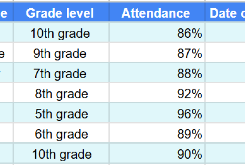Now that we've done some basic text formatting and the column widths, let's look at some of the data that's actually in our list of students here. So, for example, this attendance number is a percent. It's not an actual number. Like they haven't been the student hasn't been here in 95 days. It's a percentage. So let's make this a percent. And I would always do that by clicking the column to do the whole column. And that way, if we add new students later, it's going to apply that formatting. So I click Column C, and then I'll just click the percent button. Now, notice when I did that, when I put 95, it's going to adjust it to 95,000%. So I may need to go in and adjust so that they are the actual right numbers I was looking for. And sometimes that does happen. Depending on what kind of information you have, you may need to do some adjustments on your data. Okay, in this case, I don't really want these decimal points after they're percent. I just want it to be a whole number. So what I'll do is these little buttons here decrease decimal places and increase, so you could increase going that way or you could decrease going this way. So I'll go all the way back till I have just a whole number. The next thing we can do is we can make changes to the date of enrollment. So I mentioned this in the previous video, but I wanted to show you some more information about how this works. I'm going to click column D and then go to format and then number and then notice there's several here for date and time. So you could do both the date and the time. You could even do a duration. Here is the day of the week and the whole date all spelled out. So let's click on that one and see how that looks. Okay? I can't see the whole date now, so I'm going to use a double click here to right size it so that it'll get just a little bit bigger for me. This is one option. This is a really nice option if we're wanting to see the day of the week that the student enrolled and not just the date itself. So you have lots of options on dates, and that was under format number, and then you could just change it to a regular date or you could come down to custom date and time and make changes there. For now, I'll just do the short date, so I'll click on that and then I'll right size my column, and I'll be done. So the next thing I'd like to show you is sometimes you'll type in information in a cell, and it doesn't match the formatting of the other items in the cell. There could have been some hidden formatting that you didn't know about. So like, right here, if I type in January 22, it spells it out completely, but I really just wanted to look like the other dates. You have a couple options for fixing that. I could go back up and just highlight the whole column and make the change. Or if you're really just wanting to change one cell, you could use this button called paint format. So to use the paint format button, there's two steps. The first step is to click the cell that has the formatting you want. So this is what I want it to look like. I'm going to click on that cell, and then I'll click Paint format, and then I'll click on the cell that I want to change. So right there, and it's going to change it over to whatever format I clicked first. So it's a two step process. This is a really nice feature. Um another thing, let me show you how it works with, like, a whole row. Like, let's say I change my font color to this maroon color, and I maybe make it a little bit bigger. And then I want all of my students to have that same format. I could select the whole row, hit paint format, and then select all these other rows and it's going to change all of them. So the paint format feature is really helpful for when there's some formatting that doesn't look quite right, and you have another row or another cell that you want to mimic. You want to copy that formatting over. Okay, next let's look at text wrapping. So let's say we decide to make a new field here called notes. And in the notes field, we want to just write some special notes about the students. So I could say, Jane arrived from Louisiana last week. Or I could say, Aaron has a five oh four plan. So I could write notes about a student, but I really want for those notes to be in this column. And the text is it's dragging out over the next columns. I want to stay under this one. You could use a feature called text wrapping. So I'm going to highlight column E and then right here, there's a button called text wrapping, and the second one is wrap. So when I do that, it's going to adjust the height of the column and wrap that text around so it all fits within the confines of the width of column E. Now, if I adjust the width of column E, it's going to adjust the text as I go. I could make it a lot smaller, and then, you know, it's, of course, going to make the text even tinier. So you have that option. That is called text wrapping. Here at the top, I noticed that this doesn't match, and so I'm going to just use that paint format we just talked about. So I'll click date of enrollment and then click Paint format and then click notes, and it will adjust that so it matches. There is another feature that works really nice for tables, and it's called alternating colors. So I'm going to highlight all of the students in my um my table and then go to format and alternating colors. And then what it's going to do is right now, Google Sheets thinks that Jane is the header. But really, Jane isn't the header. She's the first student, so I'm going to uncheck that. And then notice how the rows are now just colored alternating colors. And then there's a whole bunch of different options here. So if you're really a fan of, say, purple, you could change it to purple. I like this light blue color just because it matches with the column heading we've already chosen. And then you could hit Done. And now it just makes it a little bit easier to read, especially if you have a lot of columns, which a lot of times, especially with student data, there's a lot of columns there. And so it can be a little bit difficult to make sure you stay on the correct line. And so that alternating colors is a nice feature for keeping your eyes on the right line as you're moving. One other way you can do that when you're looking at data is just to select the column. So if you didn't have the alternating colors, you could just select the column that you're looking at, and in that way, you can see exactly all of the data for that particular student. 5. Practice What You Learned: Now it's time to practice what you've just learned. So I've provided you two different documents that you can use in Google Sheets to practice. The first one has the word practice in the title, and that's going to be where you're going to create your Google sheet. And then there's a second one called solution, and this is what your sheet should look like. So you can refer to this one that I've created and try to make your practice one look like the solution as close as possible. So you'll need to enter in the column headings, enter in all the data, change the colors of the background here, change the formatting of everything you've learned so far. So take a moment now, download these two documents. This one is called solution, and this one is called practice, and try to make the practice one look just like the solution. Pause the video now and then come back when you think you're all finished. Okay, let's walk through all of the steps to make our practice spreadsheet look like the solution. Now, I'll give a little bit of a disclaimer before we go. There are a lot of different ways to do things in Google Sheets. Most of the time, there's not just one way to do it. So you're just trying to get your spreadsheet to look fairly close to mine. If it doesn't look exactly the same, that is okay. That's not a problem at all. So I'll go ahead and get started and show you how I would do it. So to start with, I'm going to look at the column heading. I noticed that that text is a little bigger. It looks like, and it looks bold. To check for sure, I could click on it, and I noticed that it's Aerial 11, and that the students' names are also Aerial 11. But this one looks bold to me. So I'm going to go ahead and make this one bold. So here's the bold button. And then I'm going to change my whole spreadsheet to Aerial 11 because when I click around, I notice that everything in here is Aerial 11. So to select a whole spreadsheet, you can click on this button right here, this little square, and that's going to select the entire spreadsheet. I'll change it to Aerial 11. Okay? The next thing I need to do is change the column headers to center. I notice that they're centered. So I'm going to select a row one and go to horizontal line and change it to center. I also need to go in and adjust the column widths. The student name looks good, the grade, the attendance, they all look fine. But the date of enrollment looks like it's not big enough, so I'm going to double click to make it bigger. And then on the notes, I'm going to just kind of drag it out, and then remember how we learned how to wrap. So rap is right here, text wrapping, and I'm going to change it to wrap so that that is wrapped. Okay. The next thing I need to do is the alternating colors. So I'm going to select all of my data. And this time, I'm going to actually select the column header as well and go to format, alternating colors. And then it looks like it was maybe this one. Yeah, that looks the same. And because I selected Row one, I'm going to choose that I did have a header here. If I had not selected row one, I would uncheck that. Okay? And then I can just hit Done. Okay, we're getting closer. Let's see what else we're missing. I do notice that the attendance and the date of enrollment are both left justified, and I would expect those to be right justified. So it makes me think maybe it's not. It doesn't think this is a percent. So I'm just going to click the format as percent button and see what happens. Okay. So it did. When I did that, it added some decimal points here, so I'm just going to get rid of those. And then maybe the case here is that it's just been left aligned. So I may need to just It says it's centered. Let's see here. I don't know. I mean, that did write alignment. It is select It is a percent now because I chose format as percent. So I think I'm probably okay there. Let's check on date of enrollment. I'm going to go to format and number, and date. And okay, it's now formatted as a date, so I may need to just write a line that as well. So that's a thing I would do on all my spreadsheets. I would just check to make sure they're formatted in the way that I expect them to be. So, just looking between these two, I feel like we're now good. I think they look to be about the same. So I'm interested to know how did you do? How did it work for you? Um, hopefully this walk through at the end helped you. Remember, when you're done, you can save your work by simply finishing. There's nothing else you need to do here. You can close these two tabs and be completely done. It's all saved in Google Drive automatically. And the way you know that is by clicking on the Cloud, where it says C document Satus and it says, All changes are saved to drive. So that's a way you can always be sure that everything that work you've done has been saved. 6. Conclusion: Alright, we've done it. In this lesson, we started in Google Drive. So remember, we started by creating a folder and then creating a new sheet by going to new Google sheets. From there, we designed our spreadsheet. We talked about basic data entry, about simple formatting. And then we had that practice where we took the practice spreadsheet and we made it look like the solution spreadsheet. So this is the best place to start with spreadsheets, and we can only build from here. In the next course, we'll dive into sorting and filtering to really help you organize your data. I hope you've enjoyed it, and I hope you'll come back soon for the next one.