Transcripts
1. Hi, welcome to the XLOOKUP masterclass: My name is Jerry. I am an excellent training and this is my class on the X. Look up functions. If you have office to 65 you only have access to this new amazing function that issue to replace yoga. If you master it, your life will be so much easier. It doesn't matter if you used you before or no, this class is for you. This training has several videos and each other videos is a self contained lessons with examples. If you would like to follow whatever doing, please download the worksheet with a central data I'm using. I hope you will enjoy this class. And I also believe that you know which of excel will bring you a job or easier and happier days work.
2. What is XLOOKUP? Do I have it?: ex Luca is a B look up replacement can do anything just like you look up, but much simpler. It can also do new stuff that was very hard or even impossible with yuca. So how can you find out if your Excel version supports X look up or no? This function was first introduced for the office 3 65 which is the subscription based version. But it is possible that Microsoft will today other versions does work. The simple steps is to just start typing the function into an empty cell. If the full name of the function shows up, then yes, you can use it. Because though we're using this function, if he goes excellent up and then share it with someone else with all the version perfect cell, then the report.
3. Before you start: Language and regional differencess in Excel: is you buy all my training. Participants come from different parts of the world. Let me explain you the differences between different language versions Before we start. All my videos are made in English versions of Microsoft Excel. However, if you use Excel in different language, which is the icons and menus are translated but also the foremost. For example, here you can see the the look of function in different languages in the ankle expression. If I start typing, if you look up, as you can see, it is recognised. If I start typing some other versions, you like German, it's not recognized and it will not work. So if you want to know the name of the former in the version off we're using for our language, Google it and Google the faction and its translation in your language. But of course, if I have an English version and you will have a German version, if I use the vehicle function and said it to you, the function gets automatically translated to your local version. Another interesting difference is the symbol separate. Most of the countries in the world used comma is a decimal separator, so my excel is set up to accept coma. So, for example, if I would like to put 1.2, I put one comma, too, and it's accepted as a number. If I will put 1.2, it will not be accepted, and in this case is you can see converted to date instead. So if you are living in a country where coma is used than your ex Ellis, most probably set up to accept coma regardless off the language versions you are using if you're living in English speaking country that you are most probably using the comma, the decimal separator as they also impact on four Morse, let's check the view. Look up for more here. We can see that there are several columns dividing the individual inputs. This is what do you use when you have decimal comma set is your separator. If you are living in an English speaking country and Oreos decimal point than most, probably you will get. Coma is an individual input separator, so into check if you use your formal us what kind off? What kind of separator does your former except if you're using this insert function way toe at it form us, then there is no difference for you. So as I'm living in a coma country, then, uh, you will see you will see a semicolons here as a divider. But be careful. Check your own so that it works for you as well, Waller. Now I have the same document opened in Google sheets. If you would like to follow this training using Google sheets, that's fine. The functions are 90% the same. Excel formulas are even 99% of same, with notable difference off the X look up function, which is, at the moment off shooting this video not supported by Google sheets, but it can change any time later. The interface is a bit different, but after you get used to it, you can work pretty well with Google sheets as well. And now I'm begin Microsoft Excel and we can get started
4. XLOOKUP intro for beginners: let me introduce you to the ex local function on this very simple example. On the travel agency sheet, I have two tables. One of them is the order list with each row representing one order of a travel agency with order I d. Customer name and the trip I d. That was selected in the other table. Have a price list with trip I d trip name and price and I will use X look upto fill in the trip name for each off the orders. So I will start like that X look up has three basic inputs and three additional imports. I will simply show you the simplest way how to use it in this video with just three inputs . So I will select strip i d. So I'm looking for that I'm interested in Is the trip name for Bradley? So the trip name off the trip I 24 Next input is the single column where your trip ideas are. Where is the index? So the function will go from the top until in finds the right grow The last of the three inputs is the return air A. This is the column where the results are so the function will check this value. Check the column G from top, and it finds the right row. It will return the results from the column H Unlike view cup. If you don't set up approximate search or exact search, the exact searches said automatically so and that's the example. As you can see, it's pretty easy.
5. Differences between VLOOKUP and XLOOKUP: the's video is for those of you that use if you look up and are interested without the differences between the look up and ex Luca. Have this example here where I found the trip name from that table using the explica function. As you can see, the imports are different, so I'm this. First input is the same looking Valka value. And then I select the search Kaloum, and the third input is the results call. And because I have a search and the results separated, it is very easy for me. Toe move around the Kolbe's as you know that, then we look up. The search column must be first in the table, and you can only look up from the columns that are on the right from the search column here . It doesn't really matter if you just switch it in the middle or at the very end, like here. The function still works. There is no problem, so we can search left with X, look up very easily, also adding new columns. It's a super easy, and it's not risky because you are counting columns in view. Look up, then adding new columns in your table might result in breaking the functions or checking the ah chicken the wrong call. So it does not happen anymore. Also, if you're sore, stable is very large and has many columns. Sometimes when we look up counting, the columns can be really time consuming. With explica, you don't have to do that. The second thing I would like to mention this video is the exact and approximate match, and you look up. You most probably used exact much all of the time or nearly all off the times. But yet you still need to set it up as an exact match to put zero or false in the very end . X look up, you can set The match is the actually is the fifth input the match mode. But if you don't set it up, it's automatically set up as exact match, which is 99% correct. So, as you can see, I didn't specify my marriage, so it will search exactly because this is what I want
6. Avoiding traps in XLOOKUP: Even though X Luca is much easier to use than Bill Cup, it still has some trips. Let me show you how to avoid those. So this is a travel agents example. We have an order list here, and we have a priceless on the other side. I would like to use the explica function toe fill in the trip name from the price list. So x, look up. I'm looking for district I d. And this is my search area. The look up array. And this is my return area. Okay? It was great. And it works. Discovery Island. Double, double, quick and well, you see here looks weird. The function of works for several lines and it just stops. It starts again and then stops Probably forever. Why is that? What I always tell my students is if you write a formula, you can be happy about it working on the first line. But that's not enough. It should work on all off the rose. So what is the problem? Let's check with the other functions are after you filled in tow Arrows You can see with every row this blue cell goes down, which is great. Yeah, we would like to search trip I d for each individual role. But will you see on the right is that also the look up array and the return l A goes down as well and we don't want that, you know, wanted to stay so, uh as we are reaching that, like is the function is not finding the results anymore because it's just simply not there . So this is not the right way how to do it, how to avoid it. Let me start again. This time I will use the absolute reference to avoid that situation. First input is the same. And when entering the seconds input to look up array, I will press before to end the dollars, you know, to use the absolute reference to avoid moving the IRA when filling the for more. The same goes for the restaurant array and that's it. Situation is avoided, but you can see the formula does not look very nice. So what I prefer in most of the cases, because in most of the cases is possible. Then I will choose full columns right there. This is not a problem at all. It makes it much easier is other side effects as well. If the price list gets longer, if there will be more trips at it, you don't have to change. The form was the foremost will adapt for the euro's automatically, so this is how to avoid it. So choosing the full columns and you'll never make a mistake for the second trip, I made a secret change in the order list in order to demonstrate it. But sure, so the ex look up starts the same to look up array, the return array. It's, it seems, to work Double Klay and not available. Not available means that the for more probable works. But just the thing that we're searching is not there. How is that possible? I'm searching for E 24 and it was found, and this e 24 was not found and everything else was found as well. Where is the problem? It happened to me several times, and now I know there is. Ah, there is a problem in the form about very often. This problem exists because there is extra space, so as you can see it lose the same. But there is extra space, which makes it different so X Look up a Samos View Cup. It's on Google. It needs to be exact match, and even the space that is extra makes it stop working. So these were two trips to still avoid using explica.
7. Looking up multiple columns at once with XLOOKUP: since the beginning of Excel. One thing was certain. A function can have several inputs, but an old photo of function is always inside one cell. Not anymore. With office to 65. When we have this dynamic for Morris, let me show you an example. With ex Luca, I would like to fill in the trip name from, ah, the price list to the order list for each off the order off my travel agency here. So I will use X look up. And, uh, I don't feel like filling up the formula twice for trip name. And that again for two price or maybe using some absolute referenced to be able to fill it to the right. So the easiest way to do right now and what you can do is select to rhetoric columns, both of them right now. So, uh what? What? It will return when you select to return columns. Both as you can see, the prices filled as well. But the firmware it's not there. It's still a result off that former. You can see this Ah, blue line around there. That means this formula spells to the other cell. You cannot edit that separately, you see is great here. You cannot edit it. So it's empty, theoretically. But this thing spilt for the error. So I would like to fill it in for all the rows. But for some strange reason, couple clicking the dot here does not work in my version. Maybe we'll get fixed very soon. But I have to use a different method tell to fill it in. Ah, I will jump to the very end and then go up. I will show you how I do that. So I will press control and the down array to jump to the very last line and the way to switch to the right side. Then I press control shift and up array to select everything in this column and press control de toe Phil down and that this felt So this is how I do that. Hopefully they will fix that soon. And maybe in your version it works with a double click already
8. Replacing error message (#N/A) in XLOOKUP: right here. I'm pointing to use extra cup toe fill in trip name based on the price list. Toe the order list for each of the orders off my little travel agency. I will show you what happens if ah, explica function will find a trip idea. It's not on the price list. For example, Trip X one. Okay, I'll change that. It's not on the list, so let's see what happens. Such for that. So, like the look up array, the rhetoric Ellery percent through and fill it in. And it is n a not available. Same like we look up. This is the way the function tells you. Uh, I've searched everything but X one. It's not there. Do something without it if you want. Nobody likes debt. Types of error in excel. Especially not your boss. So how can we specify that? How can we tell the user of our table what actually happens? That trip was not found. We can actually, with X look up very easily. Replace the error message with our own. I will show you how to do that. So I will start with X. Look up. The 1st 3 imports will be the same Look up the return, and then we have 1/4 input, which doesn't have to be put its voluntary, but it says if not found. So you put a message that will be placed in the cell if the look of value will not be found . So just put drip not found easy like that. The change in the first row with me Double click. And yes, you can see trip not found. Isn't that great? Or what? If you would like to live just like empty line if the triple isn't file. In that case, what I do is I just both the empty, uh, science like that double click. And I have empty cell. Isn't that super easy to work with, explica? I'm still amazed.
9. Looking up from a table on another sheet: I have two tables here on the sheet travel agency. It is an order list, with each room representing one order and with customer and trip I D and a price list, which shows all the trips we offer to our customers. And I use the explica function toe. Look up the trip name and the price. But the question is, does it also worker? When the stables will be in different sheets? The answer is yes. And also this is a more common way. I would actually not recommend placing tables next to each other and excel like that because, for example, if you plan to delete one of the orders, then you might accidentally delete one of the one of the trips as well. Also for filtering. If you filter in one table, Rose will be filter. It also in the other tables isn't not a good idea to put stables next to each other, so it's much better to put it in the separate cheat. And right now I did that, and I have them in separate sheets, orders and prices. So that goes toe orders together first thing before we start filling it, explica function here you need to know something about cell referencing. So if I would like to have this value here, I would just put people sign and click into that cell presenter and that this covered. And if this will change, I will get the updated information here is about So this is the simplest cell reference you can do in Excel. You can do the same even if the source is on different sheet. For example, if I post eq assign, click on prices and click here Presenter, I get the same but from a different sheet. And if I definitely to see the firm or you will see that there is ah, in our information there is equal sign. Then there is a name off the other sheet exclamation mark and the seller friends on the other sheet. So I called this like like international calling coat. So this is we're calling to different countries to put a special code. Same goes for ah, sheets. The same goes also weaken the reference thinks on in different world books actually so but this example of issue on different sheets so it can use the extra cup like that for referencing to other sheets. I like to use this insert function because it makes it a little bit easier. So let me choose X. Look up. I have it right here in my most recently used. If you don't, you can just type X, look up here and go and it's right here. Press OK? And so I will select. Look at value. So I would like to know for ah Bradley here. What is the name off the trip that he ordered? So I look like I'm looking for I 24. Look up array So I will go in prices because I need to search in this column and return. It's the result Should be from death color. This is enough for me at the moment. Click OK And I have the trip name. No, I can double click here to fill the function in. That was easy, right? But it is very easy to make a mistake while doing that. Let me show you the typical mistakes that happens here. So in their function X, look up and look up! Will you click here and now I will switch Ah, switch the sheets before I finish entering the look a value. So I still stay in this input box. Change the sheets, see what happens. Actually, the cooling coat appeared here for some reason, the plus prices, or maybe sometimes it can be replaced by that. This is something you would not work because that would not work. Is your cap value So be very careful. After you finish in putting your look at value, you need to actually click to the next input books and then switch sheets because as soon as I use which heats, the calling court will be input into your input box. So prices I will sell like the this thing. And be careful here again because if you still stand in the look up array and switched back toe orders, this will change. And now you're looking up in the wrong sheet. So after you select your look up array, be sure to click in the return array and inside written area. Be careful that the after you click in the new input now we are back in the orders once again. So they have to re click toe prices and a slightly colombe. So as you can see, there are a lot of traps in the behavior Off Excel is predictable, But sometimes let's say you would not expect it or you will. Ah, it would not be the best user friendly experience. You have to be careful when you're building a for more that you do have the international calling coat where they're supposed to be, and you don't have them where they are not supposed to be. So this is how you put ah ah Have you use, uh, ex look up across different sheets?
10. Horizontal lookup with XLOOKUP: the explica function can also do horizontal surge. Let me show you how to do that. I have a table here on this sheet called horizontal and to the match. And this table shows number of business clients per country. Each column is a country and sales representative. Each row is one says rep and there is a total role as well. Here in the bottom life, I would like to look up, wrestles for all countries. So for u K, I would like to search the total. So for UK would like to find out this number for USA right here. I would like to get this number etcetera, and I can use explica for death. You couldn't use view. Look up for that because veal cup can only search of vertically. You would have to use a H look up in this case. But extra copper places both of these functions, and it works exactly the same way. So let me put extra come here and I'm looking for UK and to look up Array is a row in this time. So this road, so it will search from starting from the A column and will search until it finds UK and the next input tells us. Okay, so after it finds UK from which row would you like to get the results, which is right here and that's it. And it works for UK quite well. But to be sure what happens if you fill it for the other ones as well, it's just not available, not found. How is that possible? When I get an error, I always double click the function to see what happens, and I can see the problem. As you can see, we forgot that as we move the function one roll down. Also, the inputs moved one road down and now they are looking in the wrong rose. This problem doesn't happen with view cup or with the vertical search because normally of searching columns and then you fill it up to rose. But this time it happens. So what we need to do is tow do the absolute reference. So I will start over and do it the correct way that works. Even if you fill in the function. So I will use X look up again. The first look of value stays the same. And now when I'm selecting to look up Array. I need to press F four in order to look it in place. You see, these dollar science will appear, which is a sign for absolute reference. That means even if I feel the function to more rose, it will stay in the same road that will do the same with Return Array right here. Selected Empress F four. And this is the correct way because it doesn't change on the first SL. But if you fill it in by double clicking to see it works and it never So this is a way how to do horizontal search using the explica function.
11. 2-dimensional Lookup - Look up both a row and a column: once we most advanced things you can do with the ex local function is two dimensional. Search here on this sheet horizontal and to the match. I have a table which is countries in columns and sales representatives in rows. And each number represents the results or number of business clients for each of the representative in each country. And here on the bottom, right, have a table, but you need to fill in. I had to get the results for individual country and individual names. So not only I need to find the right column here. I also in to find the right row in the same time. So the result for UK for Joan is currently right here for USA. It's right here. The total for France would be this number, etcetera, etcetera. So I need to search in both rows and columns. You could use vehicle for that, but need to combine into it also with to match function. It's quite tedious process in X look up. It is a little bit easier, especially thanks to the dynamic arrays, which is a new way how to use ah hell to use formulas in excel, I will show you in a second. So let's start finding the wrestles for UK for John. And if I was split it into several steps and the first step will be to finding the right column for country. So let's find the UK call in the full table. So I will make like a space here for the right column. So I was finding here. I will use X look up to look up for UK. I will look up for in this array in the list of countries, including the total and my return array will be this array. So everything I will fix it with a four once again. And as you can see the result of this form one, it's not just one cell, but it spilled into multiple cells is a new way hope toe we can work with for most in excel . So So, uh, you can see the result of the same former. It's all the former is in this cell. And even though the numbers are also outside, you can see in the address bar that the formula is great in this in the outside, off the first cell, so we can use that as an input toe form us. We will use search for the school to find the right name in it. But before we do it, I wish you that if I change from UK, for example, to us A the results in the right column will change or France So it works. So it finds all the numbers from the right. Cool. So let's find the right name in it. So I believes X look up. Once again, I would look up for John. My look up array will be here, Press it for and the return array will be the right column the output, which I have right here to select it like that. And as you can see, there's this dash. This dash means I'm not only selecting output off this style, but also include any off the cells and of the results that will spell out off this cell. And I also need to press a four to fix it in place. Click here inside and press four to put the absolutely friends on it. And this is the result I got, you know, for a different name of ST Paul. And as you can see, I get the correct result, but this is quite difficult. It works for the 1st 1 but we cannot simply fill it in because this right column is there only once we need to have this right going for, Ah, for all the roads, it's quite difficult. So what we can do instead is instead of referencing to the right column, we can take this formula right here. This explica for mother finds the right column and included in that excellent primary reference it's. Instead of referencing the right column, we will put the explica function that will find it. I admit that it can be a little bit abstract for this moment because it works with a raise and matrices. But it works. This is the way how it works, and I don't need this thing again. I can clear it, and I can easily double click and fill it in the other columns as well. And it works is you can see you can simply change it, and it works for all of the columns. So this Saad, we do two dimensional search using X look up
12. Wildcard search - Lookup a value when you only have a part of it: Sometimes you can end up in a situation where you need to look up a value in a database, but you only have a part of the value and not a full value. That would be a 1 to 1 match, but only part of it. Like in this example on the sheet called Wildcard Match, I have my order lists for my travel agency each row being one order with order I d full customer, surname and name and trip. I d off that order and it appointments. They will right here. I wouldn't have a part of the name. I actually have a surname off one customer, Mr or Mrs Bakes. And I would like to see if that person is in the database and I would like to search for its full name and his or her trip I d. You can use view cup for dead, but you can use X Look up. If you use the wild card match, I will show how that works. So first I will start a We look up justice normal. I'm looking for Mr or Mrs Bakes in a list off names and I would like to return Ah, the full name of the person and the trip I d. So Columns B and C and the next input is the value if not found. I can leave that empty for now. And the match moat. You know, there is an exact match and approximate match in Ville Cup. This time we have some other functions. One of them is also the wildcard match and this is will be search for number two is the world car correct image. Okay. And we don't have toe fill in the last inputs so that that should work like that and it was still not found because there is no Mr Bakes right now. We need to use the wild cards, actually, and we have two wild cards that we can use and you may know them from filtering in Excel or working in with files in Microsoft windows. These are Asterix, which replaces any number off characters or including no characters or a question mark which replaces exactly one character. So for Biggs, I need to put an Asterix to find that person and let me see if it works. And in the US there is a Rory Bakes with a trip. I d I 23. There could be more. Mr. Biggs is in the time we look up or ex. Look up in this case will show me only the first item found. But as these people are sorted alphabetically, I did do that before. I know that there is just one of Mr Biggs right here. But in the case, theoretically, there could be Mr Biggs Lee or something like that. So to be more exact, I would put like a coma. So this is the name comma. And there they should be the Asterix replacing any name. So this is, uh this is a little bit better. So But what? What should I do if I have just like Biggs? And maybe I have a longer list off surnames and I don't like toe put the wild cards into each of the eight times I can use. Do it like that. So when I'm putting the extra cup, I will say, OK, I'm searching for Mr Bakes. Then I use the ampersand toe glue something through it, and I will glue the remainder off for them Searching force. I'm searching for Mr Bakes, then comma and then Asterix like that and the rest is the same. So I'm looking up before in column B results should be B and C and, uh, if not found a leave empty and much more is to for a wild card image. So this is how I can do it as well. But what if I search for Mr Adam? Let me see formal at work, and I find actually Mrs at them. But I know it was a Mr Adam, so because here it searches from the top. So you will find the first value matching that situation. That while card which is Miss Denise at him being first on the list. But there's a jet of them. Uh, let me show you a different way. Helped to use explica there in a way that you couldn't use it well before. And this is you can choose if to search from top to bottom or if you would like to start your search at the bottom and go to let up. It can be useful sometimes this time, if I change it, it's actually the input. The last import of fifth input off explica function and you see the default is searching first to last, but I will put a minus one to search last to first and it will go from the bottom. And as I know, this one is a politics started. It will go from the bottom until it reaches Mr Jacque Adam. And that's correct. Let me show you some more advanced examples. For example, what if only? Well, if I know only the first name I know one of the customers. He just told me his Kyle he just send me the payments and it shows just Kyle in my bank. So how do I search for a person like that? I will use the first form a lot to show it. And I will just put Kyle, but because I don't know the first name I need to put the Asterix Mr Risk. OK? You that well No, I'm searching for Kyle with any any surname, and it works. It finds Kyle Blair and they're gonna be more Kyle's in that list differently, but you'll find the 1st 1 right here. You can do more advanced stuff with with that, For example, if you just know. Okay. That personally? No. Uh huh, Her name is Debra and her surname started would be, but I'm not sure. So I would just, like, be a streaks and Deborah and fill in the formula, and it doesn't find anybody. Why is that? Because I'm missings place right here. So, uh, Deborah Black right here we can go even more advanced. I just know. Don't know the surname. I just know it starts with B. What is the first person who surname stars would be so we could be. And this time I know it has hated four letters, so we had a person that xcar necessarily will be four letters, so that would be the thing I'm searching. So this is how we use the question more so b. And there are There were exactly three letters. So, uh, can do that. And I see the 1st 1 on the list is again Ah, Mr Kyle Blair. If I just know, just show me. Show me a person with just any surname. We just for characters like that. And that would be, I guess, Mr Blair as well. No, it's actually Denise a damn. You set the 1st 1 or would like to search a person that has four letter first name. I would use it like that. These searches would be maybe not that practical in death, particle or example I'm showing you, but I just wanted to shoot How to use this about cars, How to combine them in different situation toe find if you only have a partial information .
13. Approximate match with XLOOKUP: Let's open a sheet called Approximate Match together and let me show Ah, a case that you can solve with the X Look up by using it a different way. I have two tables here, a customer stables where I have my customers and the sales they did with our company last year. On the right side, I have a rebate stable because we have a system to instant device our customers to spend more. So if they reach some thresholds, a minimum sales will give them a rebate. And I would like to find out what is their actual a level of rebate and what is the actual absolute rebate So I can use explica for that If I would use extra cup like that. Ah, looking up in this array and returning this Ah, I will get not available, of course, because this exact number is not available in this number. So I can't use the default version off this function which is got exact match. So either it finds this exactly or get gives not available. I need to use a different match type, which is set in the fourth input of the function so that the actual fifth input of the function. The fourth input of the function is have not found that you leave empty and the match moat right here has four values. Zero is for the exact match and this is the default for ah X look up. It will be of two versions minus one and one minus one shows exact match or next small item . This is what we want. We they want tohave find this number and if it's not, there means to find the threshold. That's the toe. The smaller item the company needs to reach in order to get the sale separate minus one. And the rebate is 15%. Yes, because the minimum sales to reach it is 15%. If I double click, uh, get the results for everybody. Ah, and that I will calculate absolute rebate by simply multiplying thes two numbers. That's super easy. There is another match mode. Those, though noticed minus man and zero. There is also there's also one which is exact much or next larger a time. Let me show you what it does. It gives people higher rebate, so it finds the larger numbers. If it's a 30 milion it will say the matchup will be 20 million. So let's say it will Deadwood work in case that will be not be a minimum sales. But it will be a treasure you know, so upto. If I would say it sales up to then, this aversion would work better. If the company has a sales upto one million, they have a 5% rebate. And here, in this case, they have a sales upto 20 million. So they are reaching 20% rebate. So it depends how your data is organized. Then you can use to off the approximate match versions, either bust one or minus month. You can also use a two for wildcard character match. But we covered that in the different video.
14. Numbers stored as text in Excel explained: look at this example on the sheet customers. I have, ah, two tables here. I have a list off or dress with a customer, a D and name and customer database again customer idea name. And I would like to fill in the customer name from the database. I can use X look up to death. So I'm looking up for this. I d and I will search death coal and have a lot to get results from that column looks right , doesn't it? It was not found not available. How is that possible? This is the question. I will try to fill it in to Ah, look what the other numbers will do and they are not available as well. What does it mean? How come five was not found when I can clearly see it in the customer i d. This is a problem that happens with nudges vulgar but also X. Look up very often in excel, and it's very difficult for beginners or intermediate users to decode what's wrong. So I will show you where the problem is, and then I will explain you more about it because this five is not the same as this five. This five ISS start as a number, and this five is stored as a text string. So from extra point of view, these are different things. Let me take you toe Texan numbers sheet and tell you more about these two data types. If I type in a number in Excel, it's ah, used as a number. You can count with it. You can multiply, divide its summit. You can put a currency symbol if you want. You can reduce the number of decimals. You can work it as a number. But what if I would like to input something like my employee number? For example? What happens is that I lost the numbers in the beginning because a number clearly cannot have numbers zeros on the beginning. So they were lost. Or if I put my phone number percent through or maybe like that press enter and the plus on the beginning disappeared. Or sometimes they can even get around it it about your phone number to get around it in excel. So for some uses, like your company, I d your full number of your bank account number. These are not actually number this our texts. These are ID's so you don't count with them. You don't multiply and divide them. So in order for excel notes to work with the missus number not around them, etcetera. Ah, you need to tell Excel. I'm gonna input a text. So I will prepare this column D toe except the older anything. I am put in there as text. I do it by selecting instead of general, I hear select text so these cells are now ready to accept text. So this time, if I put my employee number I pro a presenter, it stays in the left side, which is usually a sign that this is considered a text. And it also it keeps the numbers also, it shows me this ever It says number, store this text. But don't worry, this is not an error. This is just like a warning. And because this is a text, because it's an I d. Then we don't have to worry about this error. If you want, you can click, Ignore error. So, uh, plus, if I put some phone number plus one toe +1234567 which is the phone number? Press enter and you will see that it's not changed. It's not converted. Also, uh, text strings can have unlimited number off are very long number off characters on like numbers except only supports 15 digits. So maybe if your invoice I D or company I d or a phone number is more than 15 digit that you couldn't use, Ah, number four months as well. So in that case, use a text for month, and for a number, you use number four months. So now we understand why these numbers and these numbers will never match. But luckily, there are ways how to convert text entries numbers and vice versa.
15. Dealing with "Numbers stored a text" problem in XLOOKUP: the situation that I have here on the customer's sheet is way too. Come on. I have two tables here Orders with each row showing customer I D and customer database. And I wanted to use exc upto find out the name of the customer base in the database, but it shows not available on. The reason for that is that these items are stored as numbers, whereas those are stored is text. And this is different thing for except luckily, there is a solution to that in orderto X Look up to work. I need to convert either both off these values to text or both of them toe number. What? I suggest that what I recommend is in this situation when when these are ideas and not actually numbers that account off, you should have both. As text, it is better for, ah, future use. And to avoid any problems, I'll convert these two texts. Let me show you high. I will create a new column and this column will be called arrival just not quite. And anyhow, it was just like a working column. I would just quit customer, I d maybe. And I will use the text function. To convert this to text goes like that text and this will be the value. And the second input is a text former. It's like, for example, how many digits it should have. I usually put just like a simple 00 means that it should have one digit minimum, which is the case basically converted as it is. So the result will be looking like that. You can see if I would put two zeros in that format text input. It would mean that two digits are minimum. So it would show me like 055 in this case or if I put 0.0, then there will be one mandatory decimal place. So if you just click this function and check the help, you will see more about these format values for text. But for now, we'll just like put zero, which is exactly what you want. Now I would like to replace those things with those things and how to do it. I will just cope with ease and basted here as values, values and formatting. Okay, okay. And you see, I get this error. It shows number stores text, but yeah, this is exactly what I wanted, so I will ignore the error. Now I can delete this. Go home. And as you can see, my V Look up already works on Lee not available value I see here is for ah, this row which shows zero. But that's quite clear because there is no zero in customer 80 a za number or Nora's A text . So I will delete this one. So we're done here. But maybe you're thinking OK, so we convert it numbers to takes. But is there a way to convert text to numbers? Luckily varies. So let me show you other way to solve this problem and that will be converting both off these values toe numbers. So let me go back to the original state. And now I'm making the original situation where the form or doesn't work because this one is number. This one is a text. Let me this time Soviet. By converting this table toe numbers, you may think it might be easy. You can just select those and here in the number section off the home top. Just select a number, but it doesn't work. It did not convert. The streak is the secret is whatever is written here does not show the data type off the cell, but it shows what will be the data type after you enter something new in the cell. This is a very important to know. And when you know that your life will be so much easier So I will show you what I mean. If I double click in the cell toe, edit it and press enter that we count, it is a new entry into the cell. And you see, now it is a number. And now this works because this is a number and this is a number. Uh, let me go back. So you might think that. Okay, so now I have toe klik into every single cell to convert it to number. It's definitely possible, but not recommend it is. It will be time consuming, but there is a work around for that using based special. I have number one here, which I put there before, but you can do you register writing one and press enter and I will Kobe that by pressing control and see, and then I will select these numbers I wish to convert, and I will go to home based, based special You ever just put based? It would just replace all of the numbers by one. I don't want that. I want to keep this value. So if I multiply every number which with number one which I have in the clipboard, then the valuable not change But it will re enter the value into the cell and the format will change toe number. So I will click. OK, and as you can see, the problem is solved. So this is how you convert text numbers? This is a work around or a trick that is passed from generation to generation in excel. One last thing you might think. OK, so if this one doesn't show, what is the value? How do I actually recognize that? Is it a text or is it a value? We have function for that so and the function is called is is next. And if you select any Coolum, it will show you if it's a text and falls because this is a number, because we just converted it. But if I take this same function and, uh, use it, apply for example on this pond, I will see through because this is a text. Obviously name cannot be anything else, so working with texts and numbers can be tricky. But if you know how to convert from text to numbers and vice versa, you're looking up and comparing tables will be much easier.
16. Nested function: Combining more functions with XLOOKUP: Let's open a sheep, goats, domestic functions. Together I will show a little bit advance trick helped tow. Combine X, look up with other functions. What I have here is an order list here. Each row is one order. I have a customer here trip I D and I would like to fill in a country name for each off the trips. Like which country does it go toe? I have a country's list here, which shows me country name based off the country code. And, uh, I don't have the country court directly here. That's why I cannot use extra cup to look it up. But I know that the first letter in the trip I d. Is the country code. So I was show first an easy way. And then it would be more difficult way how to do that. I will create a new column, right that pressing control pass and I will put the country code heat here. Okay, number click. And there's a function that can take any texts, drink like that and keep only one character from the left side. And the function is called left like that. This is exactly what we need By the way, if you need it more than one character, you could just simply put the next input into this function. And let's see Number two for two characters from left, they could be useful one day in some other situation. In this light, we need just one so we can leave that empty and it'll by default. Take one character from the left, and now we can find the country name use using explica. So it's look up. I'm looking for the country code here and please surges column and after find it, give me results from Death Column and now we have the country name. I will fill it in so I can see it everywhere. And that was easy. But there's a more easy, easier way how to do it. And I can combine that into one function. I don't have to, uh, link here to another cell where a function find something. I can put the function directly insight into the explica function, or double click it and I will copy the function and not including the equal sign just like that. Oh, copy that. They look like the extra couple instead, off the reference to D five. I will delete those. And so if I will place what is actually Indy five, which is a function like that. So I know I placed a function inside a function so the inside function will be done first and then the outside function will be done. After that. These are a gold nested functions, and they can work like that in. Except if I fill it in, then the advantages that I don't need the country coat anymore. So I can simply deleted by pressing control and minus. So this is how ah, the function looks like X. Look up left C five and this is how you do. Have you do Anesta faction Excel. You can combine functions in a more complicated structure. It's like a building books off your future formulas that can be even much more complicated than this.
17. Case study: Comparing Price Lists: comparing two data sets is a skill that everybody should. Master X look up is a great function to do that. What we have now are two priceless prices this year and prices last year. I would like to compare them. I would like to find out if there ever and differences for each of the items. And I would look also like to find out if there are some new items that were not included in the last years price list and I would like to see their and the obsolete item that means that are included in last year's prices. But they are not in this year's prices anymore. So let me show you how to do that in this is price list. I will make a new coal which would be called prices last year or price last year, and I will look up the price and then I will compare it and calculate the difference. Okay, let me fill in the formatting. I will use the X look, a function here. As you can see, I have it right here in my most recently use function. If you don't just type X, look up here and could go and you will see that click. OK? And so I'm looking up for this item. This first item and I want the function to go to do prices last year go through the first column as a soon as it finds the right item. I would like to get the result from the Columbia with the price. Okay. And as you can see for the first item, the price is the same last year, so alike to calculate the differences. So this year, minus last year. So this is the difference. I would just like ah, cloned the formatting, and I can double click to fill it in. Now I will use sorting toe. Find out the differences. If I click sorting smallest of largest, I will see that there are two up their items that goes cheaper compared toa last year's. There's a price decrease in these two items. Let's be sorted by difference from largest to smallest and what I see here it's interesting because it shows me not available. This is a typical error that explica function shows when the item was not found, and that gives me information that these attempts who are not found in last year's price list. That means that they are new. So if I can who I would like to put status, these would be the new high temps. Okay, not like that. I just click and drag. Okay, so these are the new items and these other price increase attempts. So what I can see here is price increase. About the increases are like, quite significant, as you can see and the out of items with price increase. If I just selected like that, I can see that there are 32 items with a price increase. And last thing I would like to know it's other any obsolete products that are not there anymore. I can't find it in that, uh, table for that, I need toe make a look up off different directions. So into goto prices last year. And I would like to search a price this year. The function is exactly the same, except the sheets are switched. So, uh, I will use explica function to look at this item. And this time I will look it up in, uh, this year's price list. The column A and I would like to get the results from column B off this year. Okay, And I don't need to come to difference We're trying to do is, uh, started from largest to smallest toe. Have the errors fold up and I will see and not available. So price this year is not available. That means these items are not anymore in this use priceless. So? So the status for them would be obsolete. So this is a super easy way how to compare to price list using the explica function.
18. Thank you, Wrap-Up, Next Steps: if you like Excel Good news. You just learn something new If you don't like excel well, with news you just learned helpful. Spend less time with it Excel is easy to learn, but it takes time to master. If you practice off from eventually, you will master it safe time. Maybe get a promotion or better job. That's for the airport before you go. Also chicken. My other excellent horses here on the bus for thanks for watching and by
 Jiri Benedikt, Future skills trainer