Transcripts
1. Introduction: Welcome to part three of this series on getting
started with RStudio. So the first part
of this series was about RStudio Cloud and how you can use different options to configure your Cloud account. The second part was all
about in polling data. And this one is about
how to clean and transform data into RStudio. So as you can see here, there are eight lessons. The first lesson, first video, is about how to select
groups of observations. So we are going to look at several functions
and we're going to learn different
order functions from especially the
deploy your package or the tidy verse package. Then video 2.3 or two parts, really two videos on how to transform a messy
data to clean data. First of all, I'm
going to define what constitutes a messy dataset
and how to clean it. So two videos, and of course, to clean a dataset, you are going to have missing
values or null values. So it's important to know how to handle missing values in R. That is the object
of this video. The next video is how to split and combine different cells. So it's using some functions to split and combines
string data. The video here is
how to combine or join or gather different tables. So it's the equivalent
of the inner join, the left or the right or the
full outer join in sequel. Finally, you're going to have
to practice video to build your confidence in cleaning and transforming data into RStudio. Of course, at the end, you can have a project
and the description of the project is under
this video here, under the project section. So I propose that we
just dive right in and learn how to clean and
transform data within RStudio.
2. Select groups of observations: Welcome to the section about
transforming data in R. So this section is
going to be all about using a package
called the tidyverse. The tidyverse is more like a
collection of packages in R, used a lot wildly
across all our users really to do data analysis
and to do also data science. The particular package
that we're going to use in this video is called the player. So first, we're going to set
the stage for this video. We're going to upload the dataset and install
and load tidyverse. And then I'm going to explain a little more of
the functions that we're going to use an R
from the dplyr package. First, we're going
to upload it in, load a dataset into
your R session, a data set called injuries. Injuries is that I said
that lists a total of 231 patients who went through the ER for
different injuries. So to upload the data
set into our project, we go to File and then
we'll get to upload. Here, we choose the dataset engineering,
and we'll click Okay. And we can see here injuries
is under Files Project. So now we can load the
data set into R session. We go to import data
set from Excel. The importer interface starts. And then we can choose our file. We can see here for
different variables in each, which is a character variable, there are several
age groups here. And then the type, motor vehicle
crashes, et cetera. This is also a
character variable and we have estimate here. You can see that RStudio guessed that it was a
character variable, but it's not actually right. Why does it say that? The reason why osteo guessed that it was
a character variable is because in the Excel data file to represent null values, we have the characters. And at the time in port, osteo is trying to guess the
data type of this variable, as you will see, is some
characters and automatically thinks that the whole variable
is a character variable. We're going to change
the datatype to numeric. So you can see here the NAs or not character and a's anymore, but are representing
null values. So we click on import
and now we're going to install the tidyverse package. Install tidy verse. Now the tidyverse is installed. The package is
important to us here, is called deep supplier. There are many
different functions in that deep layer package, but we're interested
in for functions here. First, the function select
that will allow us to select variables or select fields
or columns of the data set. Then we're going to
use the function filter that will allow us to get rows based
on certain conditions. The third function,
we're going to use this function group by that allow us to group the data set based on
a particular variable. Then we're going to use
the function summarize, to summarize the estimate
or to do a total of the estimate of the data
based on some groups. So first the function select, I'm going to show you two
ways to use this function. First, we're gonna compose the function as it's
normally written. And then we're going
to use what is called the pipe operator. Now, the point of the pipe
operators to help you write code in a way that's easier
to read and understand. It's a way to chain
different actions. I would say in our the pipe
operator that you write, percentage greater
than percentage. That's how you write it. This pipe operator comes
from the Maghreb package. But when you load,
the tidyverse loads automatically this
pipe operator, we're going to use it right now. First I'm going to
show you how to use the function as it is written. So select, the first argument of the select function
is the data set. So injuries. And then the second
function is the columns or fields or the variables
we want to set up here. Let's select age. So to use the pipe first, you start with the beginning. Right in the beginning
is the data set. So injuries. And then you
insert a pipe operator. You can also select
multiple columns. Of course, in that case, you use the pipe operator, select an agent type here come as a collection of
vectors and not just H, you want multiple columns, so we have to put them
into a collection. You can also use
the index column to select your variables. Here I'm selecting column
one and column three, so age and injury. So now we're going to
use the verb filter. And filter is used to filter the data set
based on a condition. So here we're going
to use an example. The condition is gonna
be the age group is going to be 0-17, right? So we're going to take
all the patients for which the age group is 0-17. We can also filter based
on several conditions. Let's say we want to filter
here based on the age group zero to 17 and also the
type hospitalizations. I'm going to make
some room here. And then we're going to
use the third function, function group BY here we're
going to group by age. I'm going to press Enter. You'll see that first
the result is a table. But then you can see in the metadata that
there's 11 groups. We can also group by
different variables. So here e.g. I'm grouping by age
first and then type. Well, there's 11 groups for
age and there's three types. So we live in times
three equals 33 groups. Now based on these groups, we're going to do
some calculations. Here. We're going to
summarize the data. So we take injuries
were buying agent type, and then summarize
and we'll say, Okay, I want this column to be
called total and total equals. So we assign, there are some
of the estimate to total and we don't forget to remove DNAs before doing the summation. So that's it for this video. In the next video, we're going to look at some
more function from the deep layer and tidyverse
package to join data, to combine cells, et cetera.
3. Transform messy to clean dataset Part 1: This video is about
transforming messy data to tidy data or clean data with some functions
from the tidyverse. So first of all, we're going
to clean the workspace, restart R. So here
you see there's no more variables or
object in the environment. I'm going to make some room. And now we're ready
to set the stage. First, we're going to see
the tiny versus loaded. Here we'll type in tidyverse. Click on the checkbox. And now the tidy
verse is loaded. The two packages are important. Here are the supplier and tidy. So let's talk about messy
data versus tidy data. What is a Macy data? There are three scenarios
here for messy data. First of all, the
column headers are values and not variable names. So let's look at the
data set here that is comprised in the deep
layer package called relic income is data from a
religion and income survey. So you can see here
that the column names here are not really variables and they
should be variables. The column names here are
values of income groups. So this is considered
as messy data. The second scenario here is multiple values
stored in one column. So I'm going to show you
that with a data set called TB tuberculosis from the
World Health Organization. So first, we're going
to upload the data set and you know how to do that. Now, you import
your data set here. Click on Browse, select
the data set T, Okay? And now you import the data set. So if I enter TB here, you can see in the
third column, G TRH, we have multiple values that
represent both gender and H, M and F as female
and the age group. So we need to separate
these two variables. The third scenario here for messy data where
we consider messy, that is, when variables are storing both rows and columns. So I'm going to show you another dataset from the
Weather Association. So now you know the drill. You upload the dataset,
you select it, and then you import it
into your R session. So that's what I'm
doing right now. N1 and enter the
new or object that has been created by
import interface. Whether I can see two things
in the element column, we have several values. So these are to be separated in different variables and also
across the columns here, the column names
are really days. They want to be 31. And this should really be
one column called date. So now let's use
the ER and apply functions to tidy or
clean this data set. And again, a tiny data set. What we consider a tidy data
set in R is three things. Every column is a variable, every row is an observation. In every cell is a single value. So we're using tidy
our d prioritize diverse functions to clean the data set that meet
as best as we can. This definition is
three conditions. Okay, so let's go back
to our previous dataset, the first one,
religion and income. So issued the command here
first view, rolling income. And I can see on the left the RStudio view
of the data set. You can clearly see here the income categories are
represented as columns, which is not what we want. And we can see on the
right on the console, I issued the second
command, relic income. So what we're gonna
do here is use a function from the tidyr
package called pivot longer. Now, this data set has three
variables, really, religion, income category, and the value within each
income category. To clean this data set, we're going to pivot the
non-variable columns. So all these income
categories into column called income paired
with its corresponding value. So this action is
sometimes referred as making a wider that
asset, longer or taller. We're going to use the
function pivot longer, that lengthens or
make the data taller, increasing the number of rows, like we said, and decreasing
the number of columns. Now the opposite of
pivot longer is pivot wider and we're going to use
it in the next exercise. So we take the data
set really income, and then the pipe
operator and we say, Hey, I'm going to take the
religion income that I said, and then I'm going
to pivot longer. What do I want to pivot? Well, I wanted to pivot on
the non-variable columns, which means all the columns of the data set except religion. So here we can use minus
religion or we can use the exclamation mark to
say not the column religion, then the argument names too. We're going to collapse
all these columns into a new column called let's
say income category. And then the
corresponding values in the argument, values two. And we're gonna call
it frack or frequency. You press Enter and
you can see here that all the column names have been
collapsed into one column, one variable called
income category, and the corresponding
value is in another variable
called frequency. To illustrate the second
situation of a messy data set, which is multiple variables
stored in one column. We're going to use the
dataset tuberculosis and use the function
separate to separate one variable into
multiple variables with either regular expressions
or numerical locations. Here we're going to use
numerical locations. So going back to RStudio here, we are going to view the tuberculosis that are
set here on the left. And the second command
we're going to just view that are set
in the console. We can see the third
column, GDR H, is a really comprised of two variables, a
gender variable, one character N or F, and then an age
group zero to 14, 15 to 24, 25 to 34, etc. We're going to use a function
separate to separate this column into two
different columns, sex and age group TB, and then the pipe operator. And then we'll call the
function separate on what column where the column G, D RH, and we're separating
these column GDR 8022 columns. So C for collection and
then do two columns, sex and age group. And we're saying, I want to keep the first character of the first column
would press Enter. And we have
successfully separated the GDR H column
into two columns, sex and age group. In the third video, I'm
going to show you what to do in our third situation of a messy data set
when variables are stored in both rows and columns.
4. Transform messy to clean dataset Part 2: Welcome to part two of this video in our
third situation of a messy data set
when variables are stored in both rows and columns. And a previous video, we looked at pivot longer
and separate functions. Now we're going to look
at all the functions. The function mutate
from the supplier, then pivot wider
from the title ER, and then a function that
deals with strings, STR sub from the
string or a package. Again, all these functions
are within the tidyverse. So again, if we
look at the first column, the column element, we can see that there
are several values and even variables in this
particular column. So what we'll have to do is
separate this column into multiple columns where the first element
characters are the id. The other four characters
are present the year, the next two characters
represent the month, and the next four
characters are actually variable T max teaming and PRC
P for maximum temperature, minimum temperature
and precipitation. But first, let's use
pivot longer again to collapse all the
days into one variable, day and all the values in
a new column called temp. So whether data
set, pipe operator, then control enter
to put the cursor on the next line without telling RStudio to evaluate the command. So we're pivoting
everything except element names to calling day. We're collapsing all
of these columns into one column called day. And then the associated
values into column damp. You can see here the
result when you presenter. And that was said before
in the column element, There's different variables and different values that we're
going to have to separate. So we're going to use this separate function
from the tidyr package. We're separating
the column element or separating this column
into four columns, ID, year, month, and element. So not the third argument
is the location. So the elephant first characters are the ID for the
second column. What's the next four characters? So up until the 15th
character for the year, and then 16, 17 for the month. And then arrest and put the L 21 go into the column element, calling it element again. So we're going to make some
room Control L up arrow to bring up the
previous command. And now we're going to use a new function from the deep
layer package called mutate. Mutate creates a new
column in our data set. Now in this particular case, we are creating a new column in place of this column element. And we're calling this
new column element. It's like an in place in Python. So we say mutate element, the name of the new
column equals to lower. So we're going to lowercase
every value of this column. And we'll press Enter. And you can see here every value in the column element
is lowercase. Now we're going to use mutate again to change the column date. So again, mutate,
create another column, but we're going to do an
implicit in place if you will, mutate day, we're going to
call it data same name. And the goal here is to
replace the values D1, D2, D3, D4 by the corresponding
day 1234, and changing the data type also of the column instead of
characteristics can see here, we want an integer. We're going to use a
function from the string or package CTR underscore sub, which is used to
extract and replace strings from a character vector. So STR sub and what concerns
us here is the column day. Now the next two arguments
is the beginning and the end of the string
we want to preserve. So the star is two and
the n is minus one. Then like we said, we want to convert this column
into an integer columns. So we add as integer
before the STR cell, and then we'll press Enter. We can see here
the column Day is an integer data type and we
have replaced the values D1, D2, D3 by just 1234. Now we're going to
use pivot wider. Now we've talked previously about the column
element with TMax teaming and precipitation
that are really variables, so they should be columns. So for this, we are going to use the function pivot wider to take this column and make three columns out of the
values of the column element. So the three new columns
are going to be T max, T min and precipitation PR, CP. And the corresponding
values are gonna be taken from the column temp. So control l to make some room up arrow to bring
up the previous command. So here we are
using pivot wider. So take the distinct values
of the column element and make up columns
new variables. Then the corresponding
values are from the column temp. We press Enter. And we can see here
three new columns, TMax, demean, and PRPP. So this data set is in a tidy format where every
column is a variable, every row is an observation, and every cell is
a single value. Now you may want to
reorder the columns or you want to read
of the id column. So what you do now is you just select the column you want to
in the order you want them. Here, select and then
see for collection. And we're going to
say, I want first of the year and then the
month and the day. And then team men,
TMax, NPR, CP. So here we have completed
these tidying of this data set where variables are stored both
in columns and rows.
5. Handling missing values: This video is about
missing data. So in our missing
values are missing data is represented
by the symbol N, which means non available. Now, there's a difference
between an a and NaN. You're going to see some times. And NAM means not a number. So these are impossible
values, e.g. they can't be divided by zero. And you're going to
have missing values in your data set, it's inevitable. So here in this video we're
going to do four things. First we're going
to test for missing values with the is a function. Then we're going to recode
values to missing data. So in our example we're
going to say all the values, that is 99, replace them by NA. Then we're going to use the function drop NA
from the supplier. And then we're going to replace all those ns with the median, with the replace a and f
function from the tidyverse. And for this here,
we're going to use the data set injuries, as you can see on the left
here in a column estimate, you see two NAs on the
right or in the console. In the column estimate, you can see an NA here in red. It means there is no values. So the first function that
we're going to use is, is delta N a function? And this function
returns a value of true and false for each
value in a data set. So if the value is NA, the function returns
the value of true. Otherwise it returns
the value of false. In this particular case, I want to see if the column
estimate has so many values. To access a particular
column in the dataset in R, we use the dollar sign, so injuries, dollar sign
estimate, we press enter. So we can see here we
have a few true values. So a few NA values in conjunction with
the function is N-A. Let's use the function
any to see if there's any null values in
the column estimate. So this is another
way to seek quickly if there's any null values
in a particular column. Now, want to know
how many null values is in this column estimates. So I'm going to sum or count
the number of inner values. And we can see there's 11 here. It is not uncommon to find a dataset where all the values, such as unknown or a
specific number like 999, represent any values
or null values. So in this particular
column estimate, we don't have a
certain number or character that
represent NA values. So we're going to just imagine that we have a bunch of 58, 30 like here that
represent any values. So what do you do
when you want to replace this number
by N A values? So we take our data set injuries and then we're going
to mutate in place. And we're going to
say estimate equals replace the column estimate. And in the economy estimate, when estimate a equals 58, 30. Just use NA or replace it by NA. You press Enter and
you see that in the column estimate
where there was 58, 30. Now there's NA. So all the values of 58 30 in the column estimate have
been replaced by an a. Now let's use a function
to drop missing values. We're going to use the
function drop NA from the tidy are dropped all the rows
containing missing values. So if you remember, there was 11 and their values in a column
estimate and year, if you look at the metadata
of the data set injuries, you can see that it's
a table of 231 rows. So if we drop the rows
containing missing values, we're going to end
up with 220 rows. So for this, it's very simple. We just take our
data set injuries and then drop the
NAs or press Enter. And we can see in the metadata, it's still table, of course, data set, but now
it's a table of 220 rose and of
course four columns. So for our last example, we're going to use
a function called replace ANA from
the tidyr package. And we're going to replace
the NAs by the mean, or you can replace it
by the median also. So first of all,
we're gonna do is we are going to calculate the mean. So mean of the rosette
injuries dollar sign to access the column, the column estimate here. And we can forget here that
we need to remove the NA before doing a mean
or some average, we need to remove the NAs. And what we're gonna
do here is assign the mean to a
variable called mean. As you can see here in
the global environment. And our object has been
created called mean. Now we're going to
use this mean to replace all DNAs by the mean. So we take the injuries and
then we mutate in place estimate equals replacing
the column estimate. And we replace the
NAs with a mean. We'll press Enter and
we can see here that the NA has been
replaced with a mean. So that's it for this video on how to handle missing data NR
6. Split and combine cells: This video is about
how to split and combine cells and columns in R. So we already used the
verb separate from the Tidyverse to separate two columns or two
split two columns. What we're gonna do is first we are going to
combine two columns. And for this we're going to use the verb or the function unite. I have uploaded
here an Excel file. You can see student grades
dot XLS that contains grades about 100 students
in math and physics. So I have uploaded and also imported the data set
that I called SD. You can see here there's
100 observations or 100 students and
three variables. The idea of the student, the last name and first name. Now if I type the R object S T, we can see here that in the column LastName
and first-name, there is a whitespace
after each name. Now, depending on the format
of the resulting column, will have to trim
all the names here. So get rid of the whitespace. And instead of using
the STR trim from the tiger on last name and
then on the column firstName, we're going to use a
function called across. And what we're going
to say, I want to trim all the names in
these two columns. So we're going to mutate in place across these
two columns here. So the data set S, t, and then I'm going to mute it
in place across two columns across and then collection of
the columns that you want. So last name and first name. Then the function
that we want to apply across is STR trim. So we can see that we have successfully trained
us to columns. Now we're going to combine those two columns
with a separator. So now we're using the function unite that combines
those two columns. We're going to call
this new column name and then columns that
we want to combine. So see lastname, firstname, the separator comma space. And then we're saying,
I don't want to remove the column last
name and first name. So here we have
successfully combined first and last name into
a brand new column name. And of course we can use
the functions separate, which splits the column name
according to a separator. So bring the previous
command and I add separate, separate the column
name into two columns. Last, first. Now say Do not remove
the column name. So in this video we've
used several functions mutate in place across
different columns. We have trimmed some columns and we have United
or combined columns, separated or split columns. In the next video,
we're going to use the different joints that are available in the dplyr package.
7. Join data from different tables: So in this last video
of this section, transforming data in R, we are going to go over the different joints
that are available in, are the different joints are part of the
supplier package. Within the Tidyverse. Here on the left you have all the functions here
you can see inner join, left, join, right
join, full join, etc. Now on the right,
I wanted to show a diagram of what it
means for the inner join. When you join table
a and table B, the inner join is going to
find the common elements. Well, the left join of a and B, the result will show all
the rows of colon a, even if there's no
commonality with table be. Right join is the opposite
result of a right join of table a and table B will list
everything from table B, even if there's no
corresponding value in table a. And the result of a
full join is going to list everything from
table a and table B. So I have uploaded here
another Excel file, student grades too, and we're
going to import it. Now. I go to Import and
then Excel file. Then I click on Browse, and I choose my file. Now click on open. When you
click on the arrow here, you can see there's
two different sheets. One for student student IDs and names, and one from grades. So we're going to use
the importer twice, one for IDs and one
for the grades. Here we can see on the left to our objects
have been created. Id with 26 observation is three variables in grades with 48 observations and
four variables. Let's look at the
ID data set here. We can see that the
student IDs starts with 100.300 here with the
last and the firstName. And if a good grades, we can see the grades for the 100 students and
the 200 students. There's no grades
for 300 students. So the commonality here
is that we have ID's and names and courses grades
from the 100 students. So the inner join is going to
show the 100 students only. So let's find out
if that's true, but using the inner join
from the dplyr package ID. Then inner join or joining with the data set grades
by the common column, which is student ID. Here we can see that only
the 100s are displayed. Let's just issue a
command to view this data set on the left up arrow to
bring the previous command. And then we add view, and then we can see the
result on the left, only the 100 students
are displayed because these are the common elements
between the two datasets. Now let's do a left join
between id and grades. And as you can see
here on the left, the 100.300 students from the IID data set
are displayed here, table B, in that case,
the dataset grades, which doesn't have any value for the courses for 300 students. So you have NA in place. Now let's do a right join. We have the opposite. We have all the student
IDs from table B. So from the grades
that I set here, and for those values
who do not exist in the data set while we
have NAs or null values. Now let's do the full join. And as I said, a full
join will show and display all the values
from both datasets and display null values
or N A values whenever there is no
corresponding value in either data set. This video concludes this
section transforming that INR, we looked at a lot of functions
here from the supplier, the tidy R N a
string or package. And this also concludes
the video course, getting started with RStudio. I hope you liked it, that
you learned a lot of things about RStudio
and the tidy verse, the DVD player, tidy our
string, our package. Now the functions
that are available to transform data into
clean datasets in R.
8. Practice 1: Welcome to practice
activity number one for the section
transforming data in R. So for this practice activity, you're going to use
the importer to import all the sheets in the
Excel file injuries. You can find the
injury Excel file data set in the resources
section in your course. Now, the name of the dataframe
should be injury dataset. Then select only cases where
injury equals assault, and select only column
injury and estimate. So now you can pause the video, do the exercise on your RStudio Cloud account
or RStudio Desktop. And you can come back
here for the answer. Now, first, use the important
to import all the sheets of injuries to click
on import data set. There's only one sheet, one data set that equal
injury data set with 231 observations
and four variables. Now of course, you need to load the tidyverse or
the dplyr package. Then you can see the R command. You take the data set
injury that I set, the pipe operator, and then you filter the injury
equals assault. So in R, there's an
equals that is in most cases used as a replacement for the
assignment operator. But that is not what we want. We want double equals here, which is always used
for equality testing. Here, injury. We want it as equals to assault
than the pipe operator. And we select the column injury
and the column estimate.
9. Practice 2: Welcome to practice activity
number two of the section, transforming data with RStudio. For this practice activity, you're going to use
the importer to import all the sheets of
student grades dot XLS, that is in the resource
section of the course. There's two sheets, so there's
gonna be two data sets. The name of the data frames
are the datasets should be students in grades respectively
for each worksheet, what I want you to
do is I want you to join the two dataframe
by student ID, the common column, and select on the the grades for salmon human. Again, you're going
to pause the video, do the exercise, and then you can come
back for the answer. So here on the left you can see I use the importer to import the data set grades with 204 observations
and four variables. And the data set students would the dataframe students with 100 observations and
three variables. Now when I look at
a data set student, I can see that for semi Newman, the student ID is 75. So I know that I'm
going to filter that a frame by
the student ID 75. But first I need to
join both datasets. I'm going to join both data
sets with a common column, which is student ID. Now, if you don't
mentioned student ID, just like here on
the arc command, the function inner
join is going to automatically see if
there's a common column. If there's a common column, then it's going to
use the column. So here in that case,
it's student ID. So it takes students
and then operator, I'm going to inner join
the students with grades, as I said, in a joint has found a common
column student ID. And then I'm going to filter
by the student id equals, equals to test the
equality again to 75, which is the student
ID of semi Newman.
10. Closing Remarks and Next Steps: So this is the end of part
three of this series, Getting Started with RStudio, this particular video course was about cleaning
and transforming data into RStudio if you missed the two
previous video courses. The first one is on RStudio
Cloud and how to set it up and use all the options to configure your Cloud account. And part two was how to import all sorts
of data into RStudio. You can look under this
video and you can find links to this previous
video courses on getting started with RStudio. And I hope you enjoyed
the course and his series on getting
started with R Studio. Thank you very much.
 Emmanuel Segui, Data Analysis Made Easy!