Machine Learning: K-Means Clustering

1. K-Means Clustering Introduction Video: Everyone and welcome to my latest cores machine-learning with k-means clustering in Python. So who am I and why should you listen to me? Well, my name is the lazy programmer and I'm the author of over 30 online courses in data science, machine learning in financial analysis. I have two master's degrees in engineering and statistics. My career in this field spans over 15 years. I've worked at multiple companies that we now call Big Tech and multiple startups. Using data science, I've increased revenues by millions of dollars with the teams I've lead. But most importantly, I am very passionate about bringing this pivotal technology to you. So what is this course about? This course is all about teaching you one of the foundational algorithms and machine learning, known as k-means clustering. This is an example of an unsupervised machine learning algorithm. Meaning it is meant to be used on datasets which do not have labels. This course focuses on teaching you how the algorithm works and helping you achieve a solid understanding by implementing at k-means yourself. 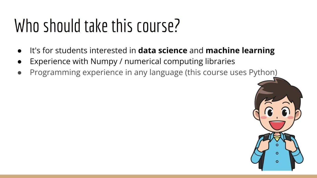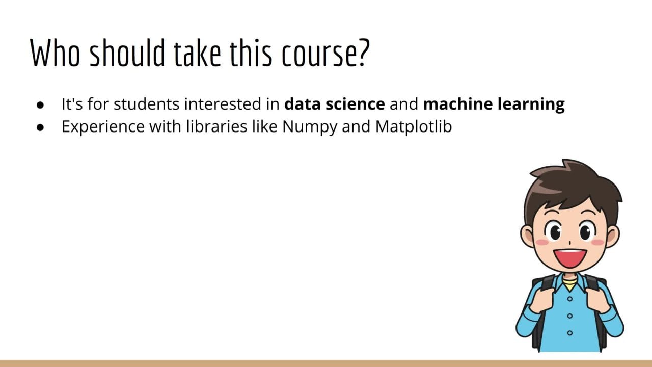These skills are critical if you want to do data science and machine learning in the real-world. So who should take this course and how should you prepare? This course is designed for those students who are interested in data science and machine learning and already have some experience with numerical computing libraries such as NumPy and Matplotlib. Note that this also implies that you have some experience with vector and matrix math, which will be used in this course. The second skill you'll need is some basic programming. Any language is fine, but since this course uses Python, that would be ideal. Luckily, Python is a very easy language to learn. So if you already know another language, you should have no problem catching up. And for both of these topics, or high school level understanding should be sufficient and an undergraduate understanding would be even better. So in terms of resources, what will you need in order to take this course? Luckily, not much. You'll need a computer, a web browser, and the connection to the Internet. And if you're watching this video, then you already meet these conditions. Now, let's talk about why you should take this course and what you should expect to get out of it. Well, simply put, K-means clustering is one of the major algorithms covered in any machine learning curriculum. It is foundational, whether you work in finance, biology or any other field which involves analyzing data. K-means clustering will be a useful tool. By the end of this course, you'll have learned enough to go out and use what you've learned on real-world datasets. So I hope you're just as excited as I am to learn about this amazing algorithm. Thanks for listening, and I'll see you in the next lecture. 2. An Easy Introduction to K-Means Clustering: In this lecture, I'm going to introduce you to the intuition behind K-means clustering and how it works. So firstly, we know that since this is a machine-learning algorithm, we're going to be working on data. So let's try to visualize some data we might get. The first thing you'll notice about this data is that all these points are the same color. This is because we're doing unsupervised learning. So there are no classes given to these points. Each point is just the vector, and that's all we know about each point. We don't know if it should be red, blue, or otherwise. But there's one important feature of this set of data. What do you notice about it? Well, our human pattern recognition abilities allow us to immediately see that there appear to be three groups of data here. In other words, we don't need the dataset to tell us that these three groups are distinct. Our own pattern recognition abilities allow us to see this very clearly. That's what we mean by unsupervised learning. It's unsupervised because nobody needs to tell us the answer. This is a key concept behind artificial general intelligence as well. If we're going to build an AI that can navigate the real-world. Practically speaking, it probably has to have some general intuition and pattern recognition ability since it would be infeasible to provide it with training data for every possible situation it could encounter. So that's a very important point. We're using our own pattern recognition abilities to tell these clusters apart. It's not in the data itself. But now you may have noticed that what we just looked at was a very unique and very specific situation. The first limitation of this data that it was two-dimensional. This is of course necessary because if we had, say, a 100-dimensional dataset, you wouldn't be able to see it. The universe itself only has three dimensions of space. So that's all you can see. Sometimes I get students that are not convinced of this fact. So if you're convinced that you can see beyond three-dimensions, try drawing a ten-dimensional cube and see what happens. Now. Why do I mention this? Well, most real-world datasets are not two-dimensional. Therefore, you can't see most real-world data. And hence, your own pattern recognition skills are not useful in this scenario. It would be nice if we had some algorithm to find clusters are groups of data that could work no matter what the dimensionality of the data is. Of course, That's what this entire course is about. So you can be confident, you know the answer to this question by the end of this course. Here's another issue. In the original data I showed you. I generated it so that it would show three distinct clusters very clearly. But what if our data looks like this? Or what if our data looks like this? Now you can see the clusters are not so clear cut. In general, we'd like to know, is the cluster I found good or not? In this course, we'll answer this question as well. So as a first step into understanding k-means clustering, Let's consider two sort of fundamental truths about the clusters in the dataset. Suppose I'm told that these yellow, purple, and green points are the centers of some clusters. And I'd like to know which Center does this new blue point belong to? And I think it makes intuitive sense that this point of course, belongs to the center that is closest to. So to decide which cluster a data point belongs to, I pick the nearest cluster center. Pretty intuitive. Let's now consider the second fundamental fact about clusters. Suppose I'm told that these data points you see here all belong to the same cluster. Let's call them X1 to X C. We'd like to know what is the centre of this cluster. Of course, that's just the mean of all these data points. This is also called the centroid, if you're thinking geometrically. And as you know, the way to find the mean of a set of vectors is to add them up and divide by the number of vectors. That's how you find the cluster center. The big question, we have these two fundamental facts about clusters. Is there any way that we can combine these two ideas to give us a clustering algorithm. Now believe it or not, these two fundamental facts are all you need to implement K-Means clustering. It turns out if I initialize the cluster centers randomly, then if I just repeat these two steps over and over, I'll converge to an answer. So just to recap, we start out by picking some random points as our cluster centers. Then I can use the fact that each point in my dataset just belongs to the cluster whose center is closest to. So I assign all my data points to their nearest cluster center. Then, now that I know each data point belongs to a cluster, I can calculate new cluster centers based on all the points that belong to it. Then I go back to the first step, which is assigning data points to the new cluster centers. Again. Later in this section, we'll see visual demonstrations of how the cluster assignments and cluster centers evolve over each iteration. Let's recap this lecture. Since while it was quite sure there was some very important ideas introduced. First, we talked about the fact that sometimes it's really easy for us to see clusters. We don't need the dataset to tell us the label for each data point. We can easily see which data point belongs to which cluster. That means we've learned to understand the data in an unsupervised way. Second, it's important to understand the ways in which that example was limited. Sometimes the boundaries between the data might not be so clearly defined. And more often than not, we won't be able to look at our data because our data won't be two-dimensional. So what we would like to have is an automatic algorithm that can find clusters for us given any arbitrary dataset. Finally, we looked at two fundamental facts about clusters. The fact that each point should be assigned to the cluster it's closest to. And the fact that each cluster center should just be the center of each point that belongs to it. We saw that when we combine these two facts together, we get the k-means clustering algorithm. 3. Exercise: Finding Cluster Centers: In this lecture, we're going to jump right in and to exercising your coding skills. This course is designed to be a hands-on course. So for every topic you'll learn about, you will implement it in code. As my saying goes, if you can implement it, then you don't understand it. Actually, I recently discovered the famous physicist Richard Feynman said a very similar thing. He said, What I cannot create, I do not understand. So if you don't agree with me, then you also disagree with one of the most famous physicist of all time. Okay, so how can you practice what you have just learned? Well in this lecture, your exercise will be to implement one part of K-means clustering. So here's the exercise. First, you're going to generate a random synthetic dataset called x. As you recall, for machine-learning, x should be two-dimensional, n by d as the number of samples and d is the number of features. You're also going to create a one-dimensional array of cluster identities called the why. Why should also be of size n, the number of samples. This is because for each of the samples, you're going to give it a cluster identity. Remember that these must be integers from zero up to k minus one inclusive, indicating that you have K clusters in total. So e.g. the first X might belong to cluster zero, the second X might belongs to Cluster one and so on. Now, how you create this data is totally up to you. You can make the data randomly or you can try to generate data which is appropriate for clustering. Personally, I would opt for the latter since the result will make more sense and it will be more visually pleasing in the end. Let's say for our example that n equals 300, d equals two and k equals three. This means your cluster identities will take on the values 01.2. I would suggest making it so that your data are evenly split amongst the three clusters. So you'll have 100 data points belonging to cluster 1100 data points belonging to cluster 2.100 data points belonging to cluster three. Okay? So once you've generated the data, what do you do with it? So to recap, what we have so far is x, which is of size n by d, and y, which is of size n. The next step, which is the centerpiece of this exercise, is to calculate the mean of each cluster. So what does that entail? Well, let's suppose I have three clusters, so k equals three. Then what you have to do is loop through each of the cluster values. That's 01.2. For each of these clusters, find every data point that belongs to that cluster. So for the sake of this example, suppose you choose cluster zero. So you want to find all the data points in x which belongs to cluster zero. As you recall, that information is stored in y, then you want to find the mean of all these data points. As an exercise, think about the size of the result. I'll give you a minute to think about it or you can pause this video until you have the answer. Okay, So what is the size of the mean vector of all the data points that belong to a specific cluster. Well, remember that all of our data points are feature vectors that live in a d-dimensional space. In our example, d equals to simply put, the mean of a bunch of d-dimensional vectors is still d-dimensional. In other words, this simply means that you have a bunch of data points and you want to find the data point which is at the centroid or the center of mass. And of course, doing this is just a matter of adding up all the vectors and dividing by the total number of vectors. Okay? So now let's suppose that for each of the k clusters, you calculate the d-dimensional mean vectors. This means that you have k vectors, each of size d. Of course, you can store this in a two-dimensional array of size k by d. So that should be the result of this exercise. A k by d matrix that contains the d-dimensional mean vectors for each of the k clusters is our desired output. Let's think of this problem in a different way, just in case you didn't understand it the first time. Okay, So suppose we have n data points, X1, X2, all the way up to x n. Each of these axes is a d-dimensional vector. Furthermore, we have n, the corresponding cluster identities Y1 and Y2, all the way up to YN. Each of these y's is an integer which can be zero up to k exclusive. Remember that if we combine all these x's into a single matrix, a big X, that was the n by d matrix I was referring to earlier. We can do the same thing to all the y's to get a big vector y of length n. Let's make this example a little more concrete. Suppose that Y takes on the values you see here. So Y1 equals zero, Y2 equals one, Y3 equals to y four equals one, y equals two, y equals zero, Y seven equals zero, y equals one, and y nine equals two. It should be clear that n is equal to nine. Now, your job is to find the mean of all the x's that belong to each of the clusters. For cluster zero, you have to find the mean of X1, X6, X7. That's because E1, E6, and E7 are zero. For cluster one, you have to find the mean of x2, x4 annex eight. That's because Y2, y four, and y are equal to one. For cluster two, you have to find the mean of X3, x5, X9. That's because Y3, Y five and Y nine or equal to two. Let's call these means m1, m2, and m3. Logically, these should all be d length vectors, since they're just the average of D length vectors. Finally, you should combine these three mean vectors into a single matrix of size k by d, where in this example, k is equal to three. And remember that the data we will use for this exercise will be randomly generated by you. As mentioned previously, you can make it completely random or you can make it look like data, which is appropriate for clustering. Now you might ask, why can't we use real data for this exercise? This is an important question for beginners. Remember that all data is the same. Therefore, this exercise would be the same no matter what kind of data we use. Generating the data yourself ensures that you understand the shape and nature of the data, rather than simply loading in some CSV. Therefore, this requires greater understanding, which is good. Furthermore, since we have many real-world practical datasets used elsewhere in the course. Now is not the time for that. Now I want to be clear that we're not doing any machine-learning just yet. This is just a very simple programming exercise to get you warmed up. All we're doing is a bit of geometry, and I hope you'll agree with me on that. We're saying, Here's a bunch of data points, and each of the data points belongs to a different group. Now find the average of each data point within each group. Okay, so I hope you'll agree with me that this is just a simple geometric programming exercise. And there's nothing to be afraid of at this point. As a bonus, since our data is two-dimensional, we can also plot it on a two-dimensional grid. So your second job is this. First plot, all of the data on a two-dimensional grid using the scatter plot. In this scatter plot, you should also color-code each data point according to the cluster identities stored in the array y. It doesn't matter what the actual colors are, just that every data point in the same cluster should have the same color. Finally, now that you have the means of each cluster, you should also plot the centers of each cluster on the same scatter plot. You should use a different style so you can differentiate the cluster centers from the actual data points. As you can see in this plot, I've used stars. Okay, so that's exercise number one for k-means clustering. Good luck, and I'll see you in the next lecture. 4. Solution: Finding Cluster Centers: In this lecture, we're going to look at the solution to the previous exercise, k-means exercise number one. Note that currently I will not provide the code for this exercise since it is very short. And because your job in this course is to learn how to code by yourself, that includes typing, designing, and getting the syntax right. At the very least, you should be able to copy what I do, although I do not recommend doing that. If you are doing the exercises as instructed, you should have zero need for a code file containing the solutions to these exercises. Typing on the keyboard builds muscle memory, which is an invaluable skill to have when coding. If you have a legitimate reason as to why you cannot type the code by yourself, please let me know and I will do my best to accommodate you. Okay, so let's get started. First, we're going to import numpy and matplotlib to standard libraries for numerical computing in Python. Next, we're going to set our configuration parameters. As mentioned previously. This means that the dimensionality of the data is to the number of clusters is three, and the number of data points is 300. Next, we're going to create the data. This is perhaps the most challenging part of the script. So let's talk about what we want to do at a high level. First, the basic idea is I want to have three Clouds of data points so that each cloud can be considered a different cluster. This is the picture you should have in your mind when you think about clustering. So how can we generate such clouds? Well, one possible idea is to draw samples from three different Gaussian distributions, each with a different mean. As you recall, a Gaussian distribution is characterized by its mean and covariance. The mean will tell us where the Gaussian is located. And the covariance will tell us how the data points from the Gaussian would be spread out. So let's start by defining three means corresponding to the three Gaussians. Will say that mu one is 00, which is at the origin, will say that mu two is 55. And we'll say that mu three is 05. Next, I'm going to create an N by D array called x. This is where we will store the data to populate x, we'll start with the first 100 points, as you recall, the colon. And then the 100 means select the indices from zero up to 100. Then on the right side, I say generate an array of size 100 by d from the standard normal, and then I add a mu1. This results in 100 data points with dimension two centered at mu one with identity covariance. Next I'm going to do the same thing. But for the next 100 data points, this time the indices will be from 100 up to 200. And on the right side, the data points will be centered at mu two. Finally, we'll do the same thing for the last 100 data points, for the indices, 200, 300. These data points will be centered at mu three. Next, I'm going to create the array y, which tells us the cluster identity corresponding to each of the axes. Since we just created the axis and they are all in order, the structure of Y is very simple. It's just 100 zeros followed by 100 1's followed by 100 twos. As you recall, if you create a list and multiply it by an integer, it's simply repeats that element of the list that many times. Then when we use the plus operation on these lists, the result is the concatenation of the lists. And lastly, we cast the result to a NumPy array. Since it's easier to work with NumPy arrays, compare two lists. Note that although our data has a special structure with all the clusters in order, the subsequent code does not assume this. In other words, the code we are about to write will work with data with any structure. Okay, so the next step is to visualize the data we just created. To do that, we'll create a scatter plot by calling the scatter function. The first argument we pass in the first column of x. In the second argument, we pass in the second column of x. In the third named argument, we specify the color corresponding to our data points and we pass in y. Note that y is just a bunch of zeros, ones and twos. Using this scheme, matplotlib will decide what actual colors to assign to our data points. Of course, you can have more fine grain control if you would like to choose the colors yourself. But this is good enough for us. Okay, So hopefully this is what you expected to see. We can see that we have three Clouds of data points, and each of them is colored according to y. Next, we're going to consider the question, given a two-dimensional array of size n by d, by convention, how do I get the D size, that mean vector of that array? That is, I wanted to take the mean across each of the n samples. Now you have to be careful here, because if you just call dot mean by itself, you're going to get a single scalar, which is the mean of every single element of X. We don't want that, since what we should end up with is a mean vector, not a scalar. To get what we want, we have to pass in the argument axis equals zero, which says take the mean along the n dimension. If you pass an axis equals one, you would get the mean along the d dimension. As always, you're encouraged to try these things out for yourself so you get a better feel for how they work. Don't just take my word for it. Okay, so when we run this and we check the shape of the result, we get two as expected. Next, we're going to use what we just discovered to calculate the mean of each cluster using the cluster identities provided in the array y. To start, we'll create an array of size K by D called means. Next, we'll calculate the mean of each cluster one-by-one, starting with cluster zero. Okay, So this code is quite compact, but in fact, there are many things happening at once. If you don't understand this at first glance, hopefully you did the exercise in a way that didn't make sense to you. So you never have to come up with the same solution as I did. You just have to come up with the same answer. Your code can be completely different than mine. So as you know, code can be read from the inside out. So let's start with the most inside thing, which is y equals, equals zero. If you don't know what this does, I would recommend isolating this and printing it out by itself so you get a better understanding. Essentially what this returns is a Boolean array. As you know, equals, equals must return true or false. But since we're using it on an array, which is why the result will also be an array. Since we say equals, equals zero, the resulting array will be true in every location where y is equal to zero and false otherwise. Okay, so what happens when we index x with this Boolean array? Well, as you may have guessed, given the exercise we are doing, this selects all the elements of X where the index is true. Okay, so hopefully that makes sense. As you recall, X is an array with n rows. Why is also an array with n elements? When we say y equals equals zero, that returns a Boolean array with n elements. Then by indexing x with this Boolean array, we get back only the parts of X where the index was true. That is to say, we get only the rows of x corresponding to when y is equal to zero. Equivalently, we only get the rows of X that belongs to cluster zero. Finally, we take the mean using the mean function, passing an axis equals zero. Then we assign the resulting mean vector to our means array on the left side at index zero. Next we do the same thing to calculate the means for cluster one and cluster two. Okay, so technically this is the end of the exercise. Although it would be nice if we could visualize what we've just found. So the next step is to redraw our scatter plot. But with the cluster means we calculated previously. First, we'll start by drawing the same scatter plot we had before. Next, we call scatter again, but this time using the means array we just created. As before. The first argument is the first column of means, which refers to the first dimension. And the second argument is the second column of means, which refers to the second dimension. Next, I'm going to pass in a few additional arguments to make the plot easier to see. First, I'll pass in S equal to 500, which controls the size of the data points. This will make the mean is much larger than the data. Second, I'll pass and C equals red to make each of the cluster centers red. This will differentiate these points from my data further. As a side note, this is an example of how we can set the color of the data points in the scatterplot manually, whereas we did not choose the colors in the previous scatter plot. Finally, we'll set marker equal to star, so that instead of just appearing as a circle, the means will look like stars, which will further make them easier to see. Okay, so let's run this. Okay, so hopefully this is what you expect it to see. Each mean vector appears roughly at the center of each cluster. As mentioned, these represent the centers of mass or the centroids of each cluster. Further, we can see that they are at approximately the original Gaussian centers. One of the stars is at 00, another is at 05, another is at 55. 5. Exercise: Finding Cluster Assignments: In this lecture, we're going to jump right into your second exercise for this section. Earlier, your exercise was to take a set of data points and a set of cluster identities. Then you had to find the mean of the data points for each cluster. This time, you're going to go in the opposite direction. Now, you will be given a set of means along with a set of data points. Your job will be to take these means and these data points and find out which cluster each data point belongs to. So remember that this is done according to Euclidean distance, or equivalently the squared Euclidean distance. Note that since the squares of monotonically increasing function, whether you take the square or not, does not change the answer. That is to say, if you're comparing distances, say 2.4, if you square these, you'll get 4.16. So the relationship that two is less than four is preserved because four is also less than 16. And it's only the relative distances that matter because all you're trying to do is find the closest mean. The actual distance itself does not come out in the answer. Okay, so as before, let's think of a very simple example of how this will work. Suppose we have three means, m, zero, M1, and M2. We also have nine data points, x1, x2, x3, all the way up to X9. So what can we see? What we can see that X1, X2, and X3 are all closer to zero than they are to M1 and M2. Therefore, X1, X2, and X3 belongs to cluster zero. In similar fashion, we can see that X4, X5, and X6 are closer to M1 than they are to zero or M2. Therefore, X4, X5, and X6 belonged to cluster one. Finally, X7, X8 and X9 are closer to M2 than they are to m zero or m1. Therefore, X7, X8, X9 belongs to cluster two. So hopefully this makes sense. The challenge is to put this visual intuition in the code. Here's how your code should work at a high level. First, you're going to generate a set of means in a matrix of size k by d, just like in the previous exercise. Also, you can use the same values for n and d and k as we did previously. So n equals 300, d equals two and k equals three. Remember that d equals two is helpful because we can see it visually. Second, you're also going to generate a data matrix of size n by d. As before, you can create these matrices randomly, but it may be helpful to generate them in a way that makes sense from a clustering perspective. Either way you do it is up to you. Personally. I think it's more useful to generate the data in a structured way so that after you find the answer, you can plot the results as a sanity check. Speaking of which as a bonus, I would encourage you to plot the results with the output of the exercise. As output, you should have an n length vector, which tells us the cluster identity of each data point. So e.g. if the first x belongs to cluster zero, then the first value of your output array should be zero. Finally, I want to note that there are many ways to do this exercise. You may have heard that when you're using NumPy, it's not good to use for loops because for-loops or slow. Instead, you may have been told that it's better to use a vectorized operations. That is to say, normally you would like to find a numpy function that can do what you want all at the same time. Personally, I think that for this exercise, it's more instructive to do it with for-loops because it makes you think about what's going on algorithmically. Ultimately, whether you decide to use for loops or not is up to you. Finally, I want to reiterate that just like exercise number one, this is not quite machine learning just yet. In fact, it's just another simple programming warm-up in geometry. What we're doing is taking a bunch of data points and a bunch of centers. And we're just trying to find out for each data point which center is the closest. So I hope you'll agree with me that this exercise is just another simple geometric programming exercise. Okay, so good luck on exercise number two, and I'll see you in the next lecture. 6. Solution: Finding Cluster Assignments: In this lecture, we're going to look at the solution for k-means exercise number two. As before, please ensure that you have completed the exercise prior to watching this lecture. Note that currently I will not provide the code for this exercise since it is very short. And because it is your job in this course to learn how to code by yourself. That includes typing, designing, and getting the syntax right. At the very least, you should be able to copy what I do, although I do not recommend doing that. If you are doing the exercises as instructed, you should have zero need for a code file containing the solutions to these exercises. Typing on the keyboard and builds muscle memory, which is an invaluable skill to have when coding. If you have a legitimate reason as to why you cannot type the code by yourself, please let me know and I will do my best to accommodate you. Okay, so let's get started. So first we're going to start by importing numpy and matplotlib, same as before. Next, we initialize our configuration parameters. That's n, the number of samples equal to 300, d, the number of feature is equal to two, and k, the number of clusters equal to three. Next, we initialize three means which we'll define our cluster centers. For convenience, I've used the same means that we had previously. Next, we're going to generate the data. We start by initializing an array of all zeros called the X of shape N by D. Next, we set the first 100 points to be normally distributed centered at the mean with identity covariance. So these will go in the indices zero up to 100. Next, we set the next 100 data points to be normally distributed centered at the second mean, also with identity covariance. These will go on the indices 100 to 200. Finally, we set the last 100 data points to be normally distributed centered at the third mean, also with identity covariance. These will go on the indices 200 up to 300. Next we have our main loop, which is the heart of this exercise. This is the loop where we will assign the cluster identities. We'll start by creating an array called a Y filled with all zeros of size n. Of course, this must have size n because we need a cluster identity for each of our N data points in x. So y is the array that will store our cluster identity. Next, we loop through all n data points. As mentioned in the previous exercise prompt, there are many ways to do this, even without you having to write any for-loops yourself. However, this is not really helpful for this exercise because writing things this way helps you think about the algorithm more clearly. Okay, So it should be clear that since we're looping over all n data points, we're going to find the best cluster identity one by one for each data point. The basic idea is this. For each data point, x sub little n, we're going to loop through each of the cluster means. For each of these means, we're going to check the distance from x of little n two. That mean. We'll keep track of all these distances so we can find the one that is minimum. So if means zero is the closest, then that means the cluster identity is zero. If mean one is the closest, that means the cluster identity is one and so forth. Okay, So we'll start by initializing a variable called closest k to minus one. We use minus one as a sentinel value. This will be overwritten as we iterate through the inner loop. Similarly, we initialize a variable called min dist to infinity. Clearly this variable will store the minimum distance from x of n to all the means. By initializing it to infinity, any distance we find within the loop will be smaller. Okay, so next we loop through little k equals zero up to big K. That is, we're going to loop through each cluster center. Inside the loop, we find the squared distance between x of little n and means of k, the k eth mean. If you don't recognize why this is the formula for square distance, I would recommend reviewing the definition of squared Euclidean distance. We'll call this variable D. Next, we check whether or not d is less than min dist. Of course, the first time we iterate through this loop, this is guaranteed to be true since Mendez starts out as infinity and any finite number is less than infinity. If this condition is true, we do two things. First, we update min dist to be the current distance d. That is to say min dist is the smallest distance we have found so far. Next, we assign closest k to be the current k. And again, this means that closest k is the index of the closest cluster center we have found so far. You should be convinced that by the end of this loop, closest K will store the index of the closest cluster center and Min dist will store the corresponding distance. Thus, at this point, we can assign closest k to y, index that little n. In other words, closest k is the cluster identity for the data point x of little land. When the outer loop is complete, we will have found the cluster identities for all big N data points. So as a sanity check, we would like to plot our results. Luckily, you already know how to do this because we did this in the previous lecture. Let's run this. Okay, so hopefully this is what you expect it to see. We can see that all the data points are assigned at the correct color, according to which of the means they are closest to. That is all the points closest to 00 or one color, which looks to be purple. All the points closest to 05, or a different color, which looks to be green. Finally, all the data points closest to 55, or another color, which looks to be yellow. 7. Exercise: K-Means In Full: In this lecture, we're going to continue our discussion of K-means clustering. One surprising fact you will learn is that by doing the previous two exercises, you've essentially done 90% of the work. You may recall me saying that the previous two exercises, we're just very simple warm-ups. They were nothing but a simple programming exercises for doing some geometry. And yet at the same time, what you will see is that k-means clustering is nothing but these two simple geometric exercises repeated over and over. Earlier. At the start of this section, we stated two fundamental intuitions about clusters. Let's recall what they are. Facts number one is that the cluster identity of each data point should be the cluster center is closest to. I mean, this just makes sense. E.g. suppose we have two groups of students, ones who are very tall, say 6 ft on average, ones who are very short, say 5 ft on average. If your height is five foot 10 ", then it should be obvious that you belong in the tall cluster and not the short cluster. Why? Because you are closer to 6 ft then you are to 5 ft. So hopefully this is intuitive. So here's fact number two. The cluster center is simply the average or mean of all the data points belonging to that cluster. That also makes sense if we have five people on our group than the so-called center would be the average height of everyone in our group. Hopefully this is just as intuitive as factor number one. Moreover, you should recognize that these two facts are nothing but the previous two exercises. Earlier, I said that k-means clustering just happens to be a loop that simply repeats these two operations over and over. So what is the implication of this? Well, it means that by doing the previous two exercises, you have essentially implemented at k-means clustering already. The only thing left is to put them together. On the other hand, there seems to be a slight problem. What one might consider a chicken and egg problem. You see each of the two steps seems to depend on the results of the other. To find the means, you need the cluster identities. But to find the cluster identities, you need the means which came first, the chicken or the egg. The answer to this is called the initialization step. In this case, k-means does provide an answer for whether the chicken or egg that comes first. Basically what we do is assign the cluster centers to randomly chosen data points in x. So this is a step we do before we loop over the two steps we discussed previously. So the end result is this. To initialize K-means, we start by picking a k random points in x and assigning these to be cluster centers. Then we enter a loop. Inside the loop, we employ fax number one. We assign each data point in x to our current cluster centers. The first time this runs, those cluster centers will simply be a subset of the points in x. The output of this step is a new set of cluster identities. Then we employ facts and number two, we recalculate each of the clusters centers according to the latest cluster identities. So the output of this step is a new set of cluster centers. Then we repeat this process over and over until the algorithm converges. So how do we know when the algorithm converges? Well, it's when the cluster identities stop changing. When the cluster identities stop changing, then obviously the cluster centers will also stop changing. And there is no point in running the loop any further, since the answer will no longer change. One crucial detail you have to know about K-means clustering is this. Although the process I've just described seems pretty straightforward, it does not result in the same answer every time you run it. That is to say, k-means never finds a globally optimal solution. Instead, it's only possible to find a local optima. One simple solution to this is to simply run k-means several times and then choose the best answer. We'll define what best means later in this section. Practically speaking, this is pretty much all you can do. And in the real-world, this is just fine. So hopefully the next exercise is not a surprise. Your job, before moving on to the next lecture will be to implement k-means in code. Remember, you have already done most of the work in exercises 1.2 of this section. All you really have to do is put these two things in a loop. The basic outline of your code should be as follows. First, you're going to generate a dataset called X of shape n by d. This time, you really do want to generate a dataset that is appropriate for k-means clustering. That is to say, don't generate a dataset from just a single Gaussian with no clearly discernible clusters. Later in this section, we will look at real-world datasets. But for now, we just want to make sure that your version of k-means does what it's supposed to do. Next, you're going to initialize the cluster centers by selecting a k randomly selected points from x. Since you've created the data yourself, you can choose the values of N, D, E, and K. I would still recommend it using d equals two so that you can visualize the results. Next, you're going to enter a loop that performs the two steps we discussed previously. Inside the loop, you'll want to check for convergence. That is, when the cluster identities stop changing at that point, you should exit the loop. Finally, if you chose D equals two, you should visualize the results. You can do this by drawing a scatter plot of the data along with the cluster identities you found. Furthermore, you should also draw the corresponding cluster centers. Since you've already learned how to do this, it shouldn't be much trouble to do it again. Okay, So good luck on this exercise, and I'll see you in the next lecture. 8. Solution: K-Means In Full: In this lecture, we are going to implement k-means clustering and code. As always, I hope you had a chance to complete this exercise before watching this lecture. If not, then I would recommend that stopping this video now until you've completed the exercise. Remember that this is to benefit you are learning. So I hope you've spent some quality time on implementing this code. Actually, the third exercise should have been much easier than the first two. Since the third exercise really is just putting the first two exercises together. So hopefully you found that to be the case. Okay, so let's get started. First. We're again going to import numpy and matplotlib. By now, you are familiar with how we make use of these libraries. Next, we again set R configuration parameters. That's d equals to k equals three and n equals 300. So the data dimensionality is two, the number of clusters is three, and the number of samples is 300. Next we create the data. We start by first creating the true means mu one, mu two, and mu 31. Important factor to keep in mind is that these true means are unknown by the K-means algorithm. They're known to us because we're using them to create the data. But k-means doesn't make use of these at all. You might want to go over the code yourself to verify this fact. So as before, we're going to use the means 0,055.05. Next, we create our X matrix of size n by d. We set the first 100 points to be a Gaussian centered at mu one identity covariance. We set the next 100 points to be a Gaussian centered at mu two, again with identity covariance. Finally, we set the last 100 points to be a Gaussian centered at mu three, again with identity covariance. So hopefully you remember all this from the previous exercises. Now, you might ask, now that we are doing the actual K-means clustering code, why are we still not using real data? So this is a good question for beginners and all beginners should be able to answer this question by the end of this course, if not already. Okay, So number one, remember that we've done a good number of examples on real-world data outside of this lecture. The focus of this lecture is to implement K-Means. The kind of data that we use is irrelevant. Why is it irrelevant? Well, remember that no matter what the data is, this code for k-means clustering would not change. Therefore, there is no real advantage to using real data at this point. In fact, there is only disadvantage. So why is that? Well, that brings us to point number two, which is that using synthetic data allows us to test whether or not our code working as expected. That's an important thing and machine-learning, when you write code, you have to test whether or not it works. But you can't do that if you use your code on some unknown high-dimensional dataset. On the other hand, this is a dataset we created ourselves and it's two-dimensional, so we can see it. Most importantly, we know what the answer should be. Therefore, it's a good way to test whether or not our code is working. So hopefully you now have a good understanding about why synthetic data is important. And also, you understand that we are still going to look at real data elsewhere in the course. So you haven't lost any opportunities to look at real data. Okay, So at this point, let's plot our data so we can remind ourselves what it looks like. This time we will only plot x because that's the only thing given to our k-means algorithm, as you will see shortly. Previously in our first two Warm-up assignments, we assume that we were either given the cluster centers or that we were given the cluster identities. Now, we are in a more realistic scenario where we know neither, we only know x. However, even just plotting x by itself, we can see intuitively where the clusters should be. Okay, so let's draw our plot. So hopefully you agree that the cluster groupings are very intuitive. Later, when you learn more advanced techniques, you will understand why generating our data from Gaussian clouds is actually the ideal use case. Next, we begin the code for k-means clustering. We'll start by doing the initialization. As you recall, this involves randomly assigning the cluster centers using randomly chosen points from x. So first, we start by creating an array of cluster centers of shape K by D. That's because there are k cluster centers, each width dimension B. Next, we do a loop, k times. Inside the loop, we pick a random index from zero up to n minus one. If you're interested, you can verify that these are chosen from a uniform distribution. We call the results of this I and I is an integer from zero up to n minus one. Next, we assign x sub I to be the KF cluster center. So we take our cluster centers array and we index it at k. Next, we do our k-means loop. As you recall, this involves two steps repeated over and over. And these two steps are simply the two previous exercises you've already done. So first we'll start by setting a variable called max iterates to 20. This will set an upper limit on how many times our loop iterates. Normally, k-means converges quite fast. So you'll find that not all of the iterations are needed. Next, we create an empty array to store the cluster identities. As before, this will be an array of length n, which stores integers from zero up to k minus one inclusive. Next, for debugging purposes, I'll start an empty list called saved cluster identities to help us visualize what k-means is doing on each step, we're going to save the cluster identities on each iteration of the loop. Next we enter our loop. So I goes from zero up to max iter is exclusive. Inside the loop, we first make a copy of the cluster identities array by calling the copy function. We'll assign this to a variable called old cluster identities. Remember that this is how we will check whether or not K-means has converged. If the cluster identities haven't changed from one iteration to the next, then there's no point in continuing because if the cluster identities are the same, then the means will also be the same. Therefore, both of the two steps would result in no change. Next, we also save the old cluster identities to our save the cluster identities list. Next, we perform step one. As you recall, this is to determine that the cluster identities given the current cluster centers. Note that the first time you run this loop, the cluster centers are just random points in X. This is Y. On the previous exercises, it wasn't necessary to make the data look nice the way that I did. K-means at some point, we'll calculate cluster identities for which the cluster means are in the wrong place. So that's why I gave the instruction that you could create any x and any set of cluster means. The point was only to write working code. Okay, So basically you should recognize that this entire loop is exactly the same as what we had before. I'll go through it more quickly this time, since you've already seen it. First, we looped through all n data points. Inside this loop, we initialize closest k to minus one, a sentinel value. Next, we initialize min dist to infinity. This is so that any finite distance we calculate be smaller. Next, we looped through all k cluster means. This is because we want to find out which of these is closest to the nth data point. Inside the loop, we calculate the squared Euclidean distance between x sub n and the KF cluster center. We'll call this D. Next, we check whether d is less than the current Min dest. If it is, we save the current B as our new men dist, and we save k as our closest k. When we're outside the loop, we assign closest k to be the nth cluster identity. Next, we have step two, which was the other exercise we did. This is to calculate the new cluster means based on the cluster identities we just found. So again, you should recognize this code from earlier with a few naming adjustments. As you recall, we work from the inside out. First, we use equals equals to obtain a Boolean array telling us which of the data points belong to cluster 01 or two. Then we use this Boolean array as an index into x. Next, we call the mean function to get the mean of all those data points. And we pass it an axis equals zero, so that we take the mean along the rows. Next, we assign this to our array, which contains the cluster centers. Once we're done, step one and step two, we can check for convergence. Again, you can see we make use of equals-equals. We want to know if our old cluster identities or equal to the new cluster identities we just found as before, since the operands for equals, equals our NumPy arrays, this will return a NumPy array of booleans containing only trues and falses, true when both sides are the same and false otherwise. Note that our algorithm has only converged if all the values are true. Basically we're doing a big and statement. So we're saying if the first position is true, and if the second position is true, and if the third position is true and so on. A shortcut way of doing this is to call the np dot all function. This will return true if the array that you pass in contains all trues inside the if statement, which only occurs if the condition is true. We print out which iteration we converged on and then we call break to end the outer loop. Okay, so let's run this. Alright, so as you can see, K-means has converged in much less than 20 steps. Next, just like in our earlier exercise, we're going to plot the result of our algorithm. So let's think about this at a high level. Starting out, all we had was the array x. Yes, we had the true cluster means, but we're pretending that we don't know those. And in fact, when you think about what you would have with a real dataset, you would not know those. So our original plot was a plot of only the data without any colors and without any cluster centers. Now, after running K-means, we have more information. Now we have cluster identities, which will let us give each point in each cluster a different color. Furthermore, we also have the cluster centers, so we can draw those on our plot as well. As you recall, we earlier drew these as big red stars. Okay, so hopefully you can recognize this code from earlier. The first line does a scatterplot of the data, coloring each data point by the cluster identities. So all the points belonging to cluster zero, we'll have one color, all the points belonging to cluster one, we'll have another color, and so on. Next we call the scatter function. But this time on the means, as before, we pass in S equals 500, make these data points bigger and we pass in Z equals red to make them red. And we set marker equal to star, so they show up as stars. Okay, so let's run this. Alright, so hopefully this is what you expect it to see. This is the same data as before, but now it has colors according to the cluster identities found by K-means. Furthermore, we've marked the cluster centers with red stars. This is all information we did not have before running K-means where we only have the data itself. Next, we have a short loop to visualize the training process. As you recall, we saved the cluster identities on each step of k-means. So by plotting the data according to the cluster identities on each step, we can see how the clusters evolve as the algorithm learns. Okay, So if you want to understand this code, I'll walk through it very quickly. First, we grabbed the number of cluster identities we've stored. Note that this is variable, since we don't know how many times the training loop will go, we'll assign this to a variable called m. Next, we call the function at plt.plot subplots to set the size of the plot. The first argument sets the width, and the second argument says the height. I've chosen the number of five arbitrarily, which is large enough for me. But the important part is to set the height, which is m, times the size of the width. This is because we are going to make em a subplots and we want them all to fit. Each of the individual subplots will be five-by-five. Okay, So next we do a loop m times. Inside the loop we call plt.show subplot. There are three arguments to this function. First is the number of rows in our plot, and second is the number of columns in our plot. So we're going to have m rows and one column. That is to say, we're going to make em plots and they'll all be on top of one another. The third argument specifies which plotted is out of the m by one plots. Basically this is just I plus one, since the first value of i will be zero. Next we get y, which will be assigned to the cluster identities on iteration i. Next we call plt.show scatter passing in our data and why the current color settings. Okay, so let's run this. Alright, so hopefully this plot is useful for you to see the progression of k-means. You can see that we start with everything the same color because we initialize the cluster identities to be an array of all zeros. Then we can see that gradually the cluster separation improves. Eventually, we end up with the final cluster identities, at which point we've quit training. The important thing to notice is how the cluster identities slowly improve over each step. By setting the cluster identities in an intelligent way, the cluster identities do not get worse, only better. In later lectures, we will quantify this idea. 9. K-Means Objective (Theory): In this lecture, we're going to talk about the k-means objective function. To introduce this idea, it helps to have some experience with other machine learning models first, such as linear regression and logistic regression. So if you do, that will be very helpful. But if you don't, then try your best to follow along. So essentially, linear regression, logistic regression, and K-means clustering are all examples of machine learning. The key word in this phrase is learning. Thus, the important question to ask is, what do we mean by learning? Generally speaking, our model usually has some objective. Yes, you might say our objective is to learn, but we want to be more specific and particular. The objective is a number. In supervised learning such as linear regression and logistic regression, that number is the error. You can think of the objective, like how many errors that I make. Thus to learn is to configure your brain such that you make fewer and fewer errors. So I hope the analogy to human learning is clear. Learning is equivalent to configuring your brain or your model of the world to make less errors. In linear regression, our objective is the sum of squared errors. There are multiple reasons why this makes sense, but here is one simple reason. Linear regression is all about finding the line of best fit. In other words, we would like the line to be as close to the points as possible. On this plot, you can see that sometimes our line of best fit overestimates when it makes a prediction, and other times it underestimates. Thus, the error can actually be positive or negative. Of course, you don't want to just add the areas together because if you add a positive number and a negative number which are the same, then you will get zero. E.g. if one of the errors is plus five and the other error is minus five, plus five plus minus five is zero. And obviously you don't want the total error to be zero when your model actually made a non-zero error. Therefore, we square the errors so that they are all positive. In order to turn them into a single number, we add them together, hence, the sum of squared errors. We call this sum of squared errors or cost function. Note that there are other kinds of cost functions, such as the cross-entropy, which is used for logistic regression. However, for this course, we are primarily interested in the squared error. The next step when you are training a linear regression or logistic regression model is to figure out how to update the model parameters so that you can make the error smaller. Exactly how you do this is outside the scope of this course, but you are encouraged to learn about linear regression and logistic regression if you're curious. The important thing is to note that just like k-means clustering, this is done iteratively. That is to say we have some loop. Inside the loop, we update the model parameters. On each iteration of the loop, we hope to update the model's parameters in such a way that the error always improves. Again, how we do this is outside the scope of this course, but recognize that it can be done. Note that the analogy to human learning also makes sense in this context. You can think of each iteration of the loop as one pass through the training data. That is to say, each time you get to see the training data, your understanding of it improves such that you will decrease the areas that you make. This is true for both humans and machines. The more I practice, the more intelligent I become. Okay, So it turns out that many machine learning algorithms are trained in this way. The method is, we think of some useful cost function. Then we derive some update rule such that if we keep applying this update rule, the model improves its error. Eventually, the error converges to some minimum value, at which point you can see that you have finished that learning. In these situations, it's useful to plot your cost per iteration when training is complete so that you can verify that the training process was successful. And again, many algorithms use this method of learning. As mentioned previously, this applies to k-means clustering, linear regression and logistic regression. It also applies to deep neural networks, reinforcement learning and matrix factorization, just to name a few more examples. Okay, so that's the idea of learning and cost functions in general. But what is the cost function or the objective function for k-means? As a side note, recall that cost and objective and loss and error are all synonyms. If I ever use one of these terms in place of the other, don't be alarmed. They all mean the same thing. In any case, if you are comfortable with the sum of squared errors for linear regression, then you will also be comfortable with the cost function for k-means, which looks very similar. Okay, so let's go through this slowly so that you understand each component of the objective. First, you can see that it's in the form of a sum of squared errors. We sum over all n data points and we square the thing inside. Note that because x sub n and m sub k are vectors, we denote the Euclidean distance with double bars. This is our notation for the norm. The part that's confusing for some people is the strange one notation. This is called an indicator function. It has a value of one when the argument is true and zero otherwise. As you recall, y sub n stores the cluster identity of the nth data point. Therefore, we can interpret this as follows. Although we sum over all values of k, only one of them contributes to the cost. It's the one that is equal to y of n. And this is because y of n assigns X of n to one a cluster. Therefore, the cost is the squared distance between x sub n and the mean of whichever cluster it belongs to. So hopefully that makes sense. We sum over all n data points. For each of the n data points, we add a single square distance. The squared distance we add is the squared distance between x sub n and the mean of the cluster that it belongs to. So if x sub n belongs to cluster k, then we add the squared distance between x of n and m sub k. As a side note, you can see that little k sums from one up to big K. In the code. Little case sums from zero up to k minus one. This is just due to how programming in Python works. So just be mindful of this difference. When we're writing equations, typically it's easier to count from one instead of zero. It's also worth talking about why this objective makes sense. To understand this, we can consider some different scenarios. First, let's consider the scenario where the clusters are very clearly defined. All the data points belonging to a cluster are very close to the cluster center. Since that is the case, all the squared distances will be very small. And therefore, the total sum of squared distances will also be very small. Okay, now let's consider a second scenario. This time, the clusters are less well-defined. Now, the data points can be very far away from the cluster center. Because of this, the squared distances are larger and therefore the total sum of squared distances will be larger. The cost function does not favor this scenario because the clusters are less well-defined than before. Now let's consider a third scenario with the actual cluster assignments are wrong in this case, because the data points are not assigned it to the closest cluster center. The squared distance between each data point and the cluster center it is actually assigned to will be very large. Because these distances are very large, the total sum of squared distances will also be very large. So clearly, in order to make the cost small, we should assign each data point to the closest cluster center, thus minimizing the distance is. Note that because of the k-means algorithm, we can write the objective function in an alternative way and perhaps this one will be easier to understand. So in this forum, we no longer have to sum over k. We know that x of n will be assigned to two whichever cluster it is closest to. Therefore, the inner part of the cost is just the squared distance between x of n and whichever mean that is closest to using the square root of Euclidean distance. In this form, we take the minimum distance directly using the Min notation. Yet another way to write the k-means objective is this. We can define a quantity called the responsibility matrix, denoted by the letter R. Basically this is the same thing as the indicator function we saw earlier. But now it is a matrix instead of a function, essentially r of n k, that is, the value at row n, column k is equal to one. If x of n belongs to cluster k, otherwise it is zero. You should be able to verify that each row of our corresponding to a single data point in X contains only a single one and the rest of the values must be zero. That's because x can only belong to a single cluster. In other words, x can only have a single cluster identity. And so again, we have this situation where even though we sum over all values of k, technically in actuality, only one of these terms is non-zero and the rest are zero because the responsibility value is zero when x does not belong to those clusters. One interesting fact is that for k-means, we did not derive the learning algorithm from the cost function. All we did was start from two simple facts about clustering that seemed to make sense. Then we discovered that if we repeat these two simple facts in a loop, we would end up with k-means. To recap, these two facts are as follows. Number one, the cluster identities should be assigned so that X of n belongs to whichever cluster center is closest to. And number two, the cluster centers are just the average of all the x's that belong to it. However, using what we know about cost functions, this doesn't seem very rigorous. You might ask if linear regression and neural networks can derive their learning rules from the objective function, why can we do this for K-mean? At this point, we are not yet ready to understand how this algorithm can be derived. But if you want to learn more, you're encouraged to learn about Gaussian mixture models, also known as GMM. Gmm is or a probabilistic model, which can be seen as a generalization of K-means clustering through the lens of the GMM, you can derive the update algorithm for K-means in terms of probabilistic quantities. So if you're looking for a more rigorous derivation, that would be the next step to explore. The main point of this lecture is to understand the idea that k-means has an objective function in the first place. You wouldn't have known this only from the algorithm itself. That's why we haven't discussed it until now. The second point is that this sets us up to write more code. In particular, your next exercise is this. Take the k-means code we had earlier and add more code so that after training, we can plot the objective function at each iteration. We expect that at each iteration of k-means clustering, the objective should get smaller and smaller until it converges to some minimum value. So please write this code and confirm that this is true. Alright, so that's the exercise. Good luck, and I'll see you in the next lecture. 10. K-Means Objective (Code): In this lecture, we're going to complete the next exercise in implementing k-means, which is to plot the cost function during the training process. Once we've done this, we can consider our k-means implementation complete. As you'll see, this is just a simple modification of the code we've already written. Since we completed most of the work in the previous lecture. As always, please make sure you've completed this exercise before watching this lecture, since that is your homework for this course. In other words, don't look at the solutions for the homework before you've completed the homework. Okay, so let's get started. First, you can see that all of the initial parts of the code are the same. The inputs are the same, the data is the same. What we're interested in is the k-means training loop. So let's scroll down to that part of the notebook. Now, you may have assumed that we would have a separate function for calculating the cost, but it turns out it is simpler to compute within our training loop. Note that we are going to use the version of the cost that contains the Min operator. In this case, there's no need to do a double summation over the n samples and the k clusters. The real reason you need to sum over the k clusters is because you need to find out which cluster each data point x of n belongs to. In K-means, this is defined by the minimum distance between x of n and each of them means. However, you'll recall that we've already found this in the code. Thus, if we made a function to do this, we would be repeating the work we've already done, which would be inefficient. Okay, so let's look at the code so we can review where we've already made this calculation. First, before we even go inside the training loop, we're going to create two new variables. We have Min discs, that's plural, which is an array that will store the minimum distances for all n samples. Next, we have a list to store the costs. This is a list and not in array since the number of iterations is variable. So this is going to store the cost at each iteration. Okay, So inside the loop, let's look carefully at step number one. You will notice that we do two loops, one over the n data points and one over the k clusters. For each of the k clusters, we calculate the square root Euclidean distance between the cluster mean, the nth data point. Furthermore, you'll recall that we store this in a variable called min dist. This is exactly what we need for the cost. Therefore, all we need to do is our inner loop is complete. Simply save men disk into the array min disks. Once we have completed step one, we now have all N Min discs, which are the squared Euclidean distances between each data point and the closest cluster center. As you know, the total cost is just the sum of these. Therefore, we call the Sum function on men this to get the cost, and we store this in our list of cars. After that, the rest of the code is the same. So after we are done training, we can call plt.plot to plot the cost per iteration. So as you can see, the cost per iteration decreases on every iteration and eventually converges to some minimum value as promised. And again, let's remind ourselves why this is important. This is important to do whenever you are training a model using an iterative algorithm. Usually this involves minimizing or maximizing some objective. Therefore, you would like to plot that objective over each iteration to check that your code is working as intended. In fact, sometimes like in the deep learning, even if your code is correct, things can still fail due to sub-optimal selection of hyperparameters. So that's another reason you need to plot the cost per iteration. If you don't, then you have no idea if your model has learned what it was supposed to learn just because your code is correct. This doesn't mean the hyperparameters you chose are also correct. So the lesson is, whenever you have an iterative algorithm, it is always important to plot the cost per iteration.