Learn LaTex - The Complete LaTex Course

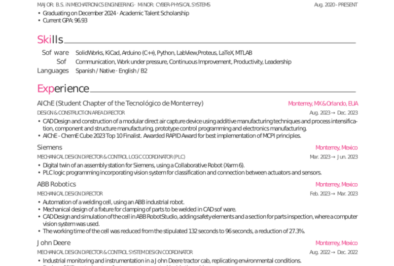
1. Introduction: So this is the complete latex course. It's a course designed to take students from knowing absolutely nothing about Latex, to being able to create professional-looking typeset documents using high-tech. So my name is Gary. I'm a postdoctoral researcher in computer science, having finished my PhD last year. And I've been working with latex for eight or nine years. So I have a good range of experience. So in the beginning of the course, where you're going to get started in the basically takes environments. So using the subsections, the different range of symbols and accents and emphasis that you can use in the latex document. And also some of the options you have for font sizes on the different lists environments. So whether you want a bulleted list or an enumerated list. We then go through including other elements into our diagrams, such as this table of contents and the figures. So using one column figures, double galium figures, and also some figures on creating our own individual figures using the tics library. So using the Takes library, we can create these really nice tree diagrams, circuit diagrams, and we can also include different tables as well. In the later part of the course, I'll give you access to some really nice templates, such as this thesis templates which you can use if you're submitting era masters or PhD thesis. It has a table of contents that has automatically updated, as well as the list of figures and tables on the different chapter titles as well. And at the very end, it also includes am, an appendix, and a bibliography gets updated. So you can also use Latex to create presentations. So I'll give you a nice Beamer template and we'll go through how you use Latex to creation, um, presentation slides. And then you'll be able to print these out to students as well. So one of the final things will go through is using latex to create CV. So latex is a good option for formatting your CV and it looks really professional and really clean. And so this course is a total, complete guide to light x. We take you through each of the individual elements such as lists and the emphasis that you can use. And then in later sections we will give you access to some really nice templates. So if you want a complete guide to Latex, you should definitely consider taking this course. 2. Installing: Okay, so we're first going to get started with installing latex. And there's a really good site called the latex project that I'll leave a link to in the resources section of this lecture. And we can use this to install all of the latest texts distributions. So this is what we use to compile our latest code. So do some slightly different distributions for Mac, Windows and Linux, but essentially all do this exact same thing. So once you have late I code that runs on Windows, it will run on Mac. And then next in the exact same way. So it's just, the different distributions are just for basically installing it on different operating systems. So if you have a Mac, you can click on the Mac OS distribution. And this brings you to Mac tech. So you can click on download mac tech, and then this brings you to the package environment. So you can download this MAC tech dot package. It's approximately four gigabytes. So it is quite large. So if you have maybe slightly slower internet connection, it might take you all and just leave it as long as it takes and it will install. So if you're using a Windows operating system, you can check out the mic TEC package. And once you go to the mic tech site, you can go to the download section. And in the download section, there is an installer here that you can download, and it's an dot EXE file. So it's really straightforward to just download it and install. They also have a mock distribution in mid-deck. But I find the previous Mac tick distribution is a bit more easier to install in Mac OS. So that's why we use dash. If you're on Linux, I assume you probably already know how to install may take, but you can get any additional information you need here using the text Live distribution. So it provides the necessary commands that you need to install it from whatever terminal you're using. So once we have her text distribution installed, we can install holder writing environment that we'll use to actually write the latex documents. So the one environment that I favor her that I been using for the last five or six years is TEX studio. So it basically just an integrated right, writing environment for creating latex documents. So it provides a lot of debugging information. There's also a lot of inbuilt commands, so you can automatically insert functions and different algorithmic environments, which we'll see later on in the course. So there's a lot of really good inbuilt options in this environment. So you can download it now. And it will automatically detect your operating system. So it's detected that on Mac and has an Alexei OSX.dmg file. So just package other console. If it doesn't automatically detect to your operating system, you can go to the Downloads file. And here you can see the Windows environment and you can download the installer and that they have here. And they've are a huge range of different latex or different Linux environments that you can download from. And if we scroll down further, it also has the Mac OS ten orders. So once you have that installed, you're all ready to get going with writing your latex documents. So in the next lecture, you will then know the latex files that we're going to be using in the course. So just one other thing to mention is that you can write latex documents online using services like over leaf. So these are really good if you're collaborating on projects, The allows you to share a link with other people, sort of like a Google Doc that you can use to collaborate on latex documents. But they can be a bit slow if you're so if you're just working on your thesis and you're the only person who's logging? Yes. They can be a bit slow compiling. So I usually prefer to have my own local version of latex and the writing environment. But if I'm collaborating on a paper or something than working on over leaf is a really good option. So in the next lecture, you're going to download these files. So for each of the sections of the course, I have a begin and an end folder. So to begin is where you start. So you see here in the first getting started with latex, we start with a totally blank document and then we build it up into this PDF. Nasa has all of the table of contents and that title sections and the different subsections I would go into. So for each of the sections, start with the begin and then work your way adding more content to this. And then if you ever get stuck, you can have a look at the end document to see what changes I've made here to create the final document. And so I also include a number of different templates, em in later sections. So we have templates for writing academic documents and also some really nice templates for and if you're writing your thesis or if you want to create your own CV. So I included tree different CV options. So some of them are quite minimalistic and there's some more modern ones. So, and this is a really nice modern one with a lot of different color. And then we also have some poster templates. So that's just a quick overview of the files. And you'll be able to download those in the next lecture. 3. Creating Our First Latex Document: So once you open the document Getting Started with latex, in that extra video, you should see something like this. So it's a totally blank document at the moment. And we're going to try and build our latex knowledge from the ground up. So the first command that we're going to learn bash is the Document class command. So the Document class commands and you can specify some key values in the square brackets. So this would be things like the font size, the size of the paper that we're using, and whether we want to have two columns, one column. So in this case, we're just going to specify that we are going to be using A4 paper. And then the class is the specific latex document you want to create. So this could be an article or report, or M, a slideshow presentation. So for these beginning tutorials, we're going to work in an article class. So once we know which type of document we want to create, we can begin a document environment. So this is something that latex expects to have an every text document. So you can use slash and then begin. And if you're using text Studio, you can see that it's providing some suggested keywords. Um, so you can use the environment name and then you get Enter. And once you hit document, you can see that creates the begin and end document. And this is because for every begin environment you alternate to end it. So TEX studio there's auto completes that force. And once we have the begin environment and begin document and an end document, we can also begin the first environment that we need for an article on this is an abstract. And now once we have our abstract environment, we can start populating it with some content. So in this case, this is a simple abstract. And now we are able to compile in few latex document. So we can use M, this green button here to compile or hit the keyboard shortcut F6. Then we can use this button to view or document or use the keyboard shortcut F7. And we can see here is her first hello world sort of latex article. You can use this green button to compile and view at the same time, or use the keyboard shortcut F5, which I'll be using for the remainder of the tutorials. And so this is a very simple document where we have the title of abstract and then just some simple text saying, you know, this is a simple abstract. So to show you some of the commands you can specify in the document class, I'm going to use a package which just generate some dummy text. So I'll explain more about this later in the further tutorials abet the different packages you can use. But this is just to show the options of the document class. So I can just generate some Lorem Ipsum text, which is just some dummy text. And you can see here that it specifies a couple of paragraphs of dummy text that we can use to, to view the options and document class. So if you want to have a document that is two column, we can just specify that in the document class options it compile. And now we have an article which is to gallium and fits onto one page. If you want to update the size of the font. So it's 10 font, but the moment I think is the default, and you want to specify it to be 12 font, an update that there. And then we see that the document goes over two pages instead of the single page. Then it was. So you can change back. And we see that the font size has been reduced again. 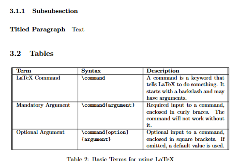4. Basic Document Spacing: Okay, so in this video we're going to look a bit more at the document spacing in my deck. So I'm just gonna go back to the default settings for the article template, which is the one column. And now we're going to add a title to her document. And so we're going to make a title which in this case is introduction to latex. And we can use in in-built command which prints the latex Logo. Are also going to specify who is the author of the document. You can specify multiple names. In this case, I'm just gonna put Gary, which is my name. And in the document just before our abstract, we're gonna make use of the Make title command. So that's backslash make title. Then we hit F5 to compile. And you can see we've got this nice introduction to latex and specifying the author and the date that it was created. So just to show some of the other m spacing options that you can do, I'm going to reintroduce the abstract, which is one paragraph text, and show you some of the different levels of sections that we can now. So the highest level section that you can have is just slash section, then you would specify your title. So in most documents the first section would be an introduction. And then if we compile dash, we see we have the number one would introduction. If you want to specify to have the section with numbers, you can use the star in after section just before introduction. If we compile that, you see the number gets removed. So just getting rid of this term, we can see that the number comes back. And then we can have different levels below this, a subsection. So that can be and learn them. And we can just populous, populate this with some lip, some text. There's another level of subsection that can go underneath as well, which is sub subsection. And this can be ipsum. So recompile this. We can see that the lorem ipsum after the first subsection, and then we have a sub sub section after this with m epsilon. So I just put one paragraph there of the dummy text. And we can see that we get the at three levels of hierarchy to ipsum. There is another level that you can go after this, which is called a paragraph. And these are usually for some small point to, to want to make her short point. And you can just say, this is a small point. And this just bowls the title of the paragraph and puts detects beside it. So when you're actually writing the text in athletic and you need to have a space between the sentences MRL set. They will be joined into the same paragraph. So this is a sentence which is still part of the same paragraph. So if you have a sentence which actually goes onto a new paragraph, you need to have a clear line of space. So this is a new era. And you can see that cuts indented and moves on to a new paragraph. So one of the things you can do with latex is to be able to refer to these sections and subsections. And the way you do that is by using labels. So when you're using labels, one good idea is to have a key in front of the label. So you would do things like SEC to specify that this is a section. If you're using tables, you'd put TAB at the front part of the label. And if you're using a figure, he'd use FID at the front part of the label. And this just makes it easier to find the references that you want to when referring to them later on the document. So in this case, we're referring to a section and the section that we're referring to is epsem. And so we specify that in the introduction. So in ipsum, we will sum in section, section epsilon, we will discuss x, y, and z. And so we can compile that. And you see it's populated with the section number, which is action 1.1.1, which is what epsilon is. And so this makes it really easy to, if sections get changed or you add, say, a subsection in front of this, it will automatically update the numbers. Just so you see this automatically gets updated to one dot one dot two because we've put in a subsection before epsilon. So this is one of the huge advantages compared to word, is everything happens automatically and later, OK, which is really useful, especially for longer documents. 5. Basic Typesetting: But one of the advantages of latex is the huge range of typesetting options or. So. In this section, we're gonna look at some of the basic typesetting options that we have. And we're creating documents and latex. So when great resource for this is the latex symbol list. So I'll give a link to this in the resources section. But basically it's a 338 page document that provides a really comprehensive list of all the different latex symbols. So you can see here we have an add different in mathematical symbols. We have inbox, some ancient languages. We have some musicals and moles. So make sure you're interested in creating some musical documents and other symbols, which can be things like clock, left arrow, right arrow, right turn, smiley face. So basically, there's just a huge amount of m symbols that are available in latex. That's never been the case that I'm I've been using latex and haven't been able to find the symbol that I was looking for. So and we're just going to take a quick look, true. One of the as sort of symbols that we can use. When you're using these symbols, you want to get the package name. So in this case we're using the mirror SIM currencies and we'll package. And so if we go back to our document, we can include that in the US package function. So the US package and then M a, R, V, o SOM. So the US package function will basically just load in these commands and make them available, available knitr document. So in this case, we can include a Euro's and MOOC. It just does backslash and then couple of E coupled UK lore. In our basic type setting section, we get our hero symbol. So you can see a huge variety of options that we have available. And seeing that we have an even multiple different Euro symbols. So we have backslash your, and then we have different, suddenly at 12345 different types of yours symbol. So we can use this slash euro HV, which maybe sounds very euro, high visibility or something. And you can see we get a slightly different Euro symbol. So one of the other things you may want to, when you're creating formulas. Later on in the course, we go through an entire section on creating equations and different formulas. But one of the things you may want even and just writing a regular document is accents. So in Tech Studio, it makes it really easy to use accented letters. So we can open up this accented land letters panel here on the left. And then we can just literary click on the Add different symbols here, different commands. And Tech Studio will automatically populate the document first. So you see here and we can have dashes because right touches left, we can have the hash and inverted hash. And if we compile this and see how it looks in our typesetting section. So you can see we have an EA with the two dots, with the dashes where a single dot when a dash going to trash can actually left the hash, the inverted hash. I'm more of a semicircular and then a straight line. So basically, every single symbol that you could try and think of will usually be available pretty easily in latex. Or you can do an online search for. And if you want to replace these with any other lenders or say a, B, and C. You can see the symbols get updated. And yeah, it looks a bit strange on the bee. But that's because B doesn't usually have these marks and vote. Yeah, so that's how you can include lots of different types of fonts and different accents in your latex document. Okay, so I'm just tidied up the basic typesetting section by adding in some sub-sections four symbols and accents. And in this subsection, we're going to look at the different kinds of emphasis. Or you can entrepreneur document. So you are probably familiar with using bold text and italicized text in Word. And we can also use these different ways of emphasis in Latex. So the way that we specify dash is by using slash text PF. And this gives us the boldfaced x. This is so bold faced x. And if we compile that, we can see we get this bolded text. So Absalom and normal text, just for comparison. We can compile Tosh and you see the difference between the bolded text on the normal to x. So we can also include some italicized text by using slash IT. And then this is awesome. Italics. And if we can combine large, you see the difference between the bolded text, normal text, and then the slanted and text that has italics. So we can also combine these options. I'm using a simple sentence. And let's say we want to bold and italicized or it's simple. So in tech studio, we can use the keyboard shortcut Command B on a Mac and Control B on a Windows machine. And then we can select where it again and command i. And that will apply. E pull phase and the italics to simple. We can see here that we get the word symbol that has been bolded and italicized and the rest of the sentence. So using a very simple air, using a parry and sentence, all are just normal text. So another formatting option that we have available to us in latex is the typewriter text. So inside some squiggly brackets, you can use backslash t, t to access the typewriter font family. And then this sample. And if we can combine lash, you see that you get this sort of monospace font that you can use for ammeter direct quotations, or by showing some algorithms. So the next way you can add emphasis or some basic typesetting to your latex document is truly use of different font size options. So in this subsection, we're going to look at font sizes. And the first way that we can create I'm really small text is by using slash tiny. So this uses a really small text size under including in the squiggly brackets to limited to this environment. So anything after such as our appendix and all these derivatives remain normal sized text. And we're only going to tiny the text inside the square brackets. So this is very small. And if we can compile up, you see that under the font sizes we get this really small text that we need to zoom into C. So if we want to come back to a normal size environment, we can use M slash begin. And then we can create a normal size environment. And inside this, we can populate it with M. So normal text. And everything compile up and see the difference now between the text sizes. So the very small and the normal text. And another way that you can type sash in latex is by using double blacks, backslash, backslash, and thus specifies that you want to create a new line after the end of this text. So we see that some normal text gets moved onto the next line. So if you want to add emphasis to a particular section of your text, you can begin a huge environment. So in the huge environment that you can do a lot of shouting and compilers. And you can see that this is much bigger than the normal text. So we can also specify the W blacks backslash. To go onto the next line. We can see here we have the various different text sizes. So these tiny, the normal and then the shedding. And so once we go right, so in this environment, we just returned to the normal text. So you can see that the text in the derivations and the additional figures has remained the same. So this allows you to specify a font options for different sections or different pieces of your document. And we also seen at the start, we can specify the default options in the document class by specifying a 1011 or 12 font. So one of the other ways that we may want to emphasize text in our document is by including different quotations. Vs. And so latex has some really good built-in environments for doing this. Hash highlights the quotation that you want to include. So we can use a slash begin. And we want to include a kosher environment. And inside the quote environment, we can basically just included the quotient. So the one I've included here is by air, Ralph Waldo Emerson. And he says that next to the originator of the sentence is the first Kosher Amish. So we can compile that. And you can see ish has increased the spacing on its side. And we've also italicize the text and giving you a dash here. And so the double backslash here again means ash. We want the text to go onto a new line. So we can show a bit of the difference here with some as seen in this. So you can see here a down some additional spacing or n, the normal text and recap the emphasis for the quotation. And we can also use some of the previous options, such as italicizing the author. 6. Figure Environment: Okay, so in this section of the course, we're going to move on to figures, diagrams, and tables in our latex document. So in this part of the course, we're going to be using the figure environment. So we can be in that she's using a backslash begin. We're going to type figure. So we'll use figure environments because they're floating environments. So instead of actually displaying the text line by line it, this will allow the figures to float to a convenient location. We can specify some placement options. But if it's in the middle of a page break or at the very end of the page. Than the floating-point environment will allow Latex to use a number of different factors and find out which is the best place to put the figure. So we use the include graphics commands to include our figures. And again, we can specify some key values. We're gonna leave this empty for diminish. And then we're going to specify the location to our image file. So the things that I like to do when I'm creating documents is to have a folder called figures. In this figures folder, we're going to keep all of our images. So this is the academies we're going to be using. We have a VGG architecture that we are going to be including with some fine tuning and some feature extraction. So there's likely they're very thin but quite tall. And we're going to be using some subclassing to include these graphics in our document. So this just keeps hear folder structure quite clean so you don't have all your images getting messed up. Wish all the auxiliary files, stock and latex generates. So once you've included the figures folder path, you can specify cash on that compile. And you see what happens when you don't specify to specify any options. Is it that the image is really big and it goes off this height of the page. So we want to specify the width on tight. And we do dash inside the square brackets. So the width and one of the commands you can use is page with sorry, line width. So if you can compile lush, ish generates the image and uses the width of the line. Because this figure environment is in two columns, it's going to use the width of the single column that it's included in. So we can also specify explicit parameters in centimeters. So say you wanted that to be five centimetres. And we can also specify the height to me, let's say 15 centimeters to make it look terrible. So yeah, you can see here the picture of the gap. The cash gets quite stretched out. So if we make it a bit more reasonable lives, five centimeters, we can see we get the square cut image here. So normally what I'm doing when I'm writing academic documents is I'll just use width and then line width. So that automatically puts it to the width that it should be for that particular line. So there's also other options that we can specify in our square brackets. So if we're going to rotate the image, we can specify an angle. And we can specify 45 degrees to get this 45 degree rotation and the image. You can also specify a negative 45 degree angle to dash D rotation for the other side. And we can also specify the placement options for latex. So latex gives a number of different and placement options that you can include in the floating-point environments. So you specify this in the square brackets beside the figure environment. So we can have it at the top, which is T. If we specify b dash and specifies it to be at the bottom of the figure, but just take away this angles so you can see that better. So if we specify B here, that says to Linux to preference placing this float the bottom of the page. We can also specify P, which is to place the image. And this places the images image on a new page and places it on a page with no extra texts. We can also specify H, which is to place it here, which is just alter this Lorem ipsum text has been generated. So D default is top, bottom place. So this is one latex will use when you don't specify any options. And I think it's a pretty good defaults. So unless you have any really good reason not to change wish, I would just leave it as it is. So one of the other things to do with figures is to add captions. So this is the text that will appear at the bottom of the figure. We can see here, it generates this text and says, figure one, this is a cash. And like the tables, we can also include a label that we can use to refer to it. And this is going to be a figure of cash. And so if we want to refer to this in the text, we can say M at the start of the figure section in the figure. And that when we refer to label someone hundreds fig, cash, cash. And if we can combine all up, you see that at the start to figures and figure one, we see a cache. So this is how we place figures. We can specify a number of different options such as the width, height, the angle, and it's a good idea 12 all of our figures in this figures folder, then we didn't have a caption and refer to them using their label. So if we want to figure to spawn multiple columns, we need to specify some slightly different figure options. So we can copy this single galium and we'll change it to big cash. That's the label so that he can compile this. We see we have the two different figures of the same size, but by placing a star in the figure environment. For both to begin on the end. And recent compiler, we see that we have a multi-volume thicker. So this is just a simple option that you can use to multicore him or larger figures to your document. 7. Subfigures: So one of the iterate types of figures that we may want to include in our document is some figures. So this is where you have a collection of different figures like figure 1A, 1B, and 1C. And you combine these into one individual figure environment. So the package that we're used to create these some figures is the subscription package. So we include that at the top. He's package, so caption. And then after the cat pictures that we've included, we can begin another figure environment. And inside the figure environment, we're going to begin another environment, which is going to require some figure environment. And so when you start to figure environment, you have to specify how much space you want. And this case we're going to use 0.16 by the text width. So the reason why we're using 0.16 is that we're using called num which 0.05. and are going to have tree individualism figure so a, B, and C. And that comes to 0.01. six, 6-7. So if you're using fair to call comes, you can double dash and you're going to treat you for the textbook. So inside the individualism figure environment, you can use the same standard commands like including graphics. And then the width is going to p t line width. And then we just specify the path to our figure, which is in the figures folders and then VGG architecture. So if you combine this, we see we have our finger here and we have room for two more figures in the same columns. So this generates some Lorem Ipsum text. So you can see this is a nuclear. So you can see here we have our figure being included in this column. So we can also specify the option of Hirsh. So it's Vdg heirarchy lecture. And as well we can specify a label that we can use to refer to this specific asset figure. So I'll just give it a label of VGG. And we can basically then include multiple of these some figures to grade the overall image. So I'm just going to copy and paste this one. And just change these names slightly so we know which one we're referring to. And then for the overall figure where you can also include a caption. So you see here, now we have our own precept and figures. And this is our collection of VGS. So they all come under the figure tree, but we've got figure a, B, and C. So I have some slightly different images. Um, so VGG for feature extraction and for fine tuning swell. So these are different transfer learning methods that you can use. So you can see that now we have slightly different images, figure a, B, and C. And then you can update the km, the captions. So VGG fine feature extraction. And this is VGG fine tuning. So if you want to refer it to each, any of the individual and figures, we can just specify them in the usual way that we referenced the labels. So as seen here on that breath. And we have the figures here. So we can specify figure a compiled up. We see that we got the correct label in defects generated after it, lorem ipsum, which is figure a tree a. So you can also specify the label for the overall figure. So just figure tree. So we can get done VGG, bigger, VGG overall. And we can then refer to that in the text as well. So we can refer to any of the individual, some figures as well as the figure over l. So that's figure tree, a tree be configure figure tree. 8. Tikz: So as we've seen, latex is really good at being able to include figures that we've generated from previous programs, either using Python or some computer graphics application. But we can also use latex and more specifically, takes environment to be able to generate our own figures in latex. So T is this. We use the package tics as t takes is really comprehensive sort of mini programming language that you can use to generate figures. So you see here, this is the documentation on takes on its one hundred, one hundred and sixty one pages on. So I'll leave a link to this somewhere in the description of this video. But it's extremely comprehensive. N goes through much of the detail of ticks. So you would really need a full comprehensive course to cover takes in its own right. So I'm just gonna give a higher level overview of takes this screen recording. So we're going to begin a new section in our document, and I'm going to call it plots. And in this section, we're going to begin our first tics picture environment. So I've just pasted some code here. And you can see that we create a ticks picture environment. And we're passing it a scale. And at this scale or passing is ten. So it's ten times the normal size that it should be. And what we're doing is we're creating a rectangle starting at position 00 and going to position 42. So that is the width by the height. And then we're drawing a line. So this is the starch, this is what we're drawing and this is the end. And this case we are drawing a line going from 00 to 0.40.2. And this case we are going from 0.20.400. So I can just remove it from the lines and show you the difference. That makes. So in this case we're just getting our empty rectangle. Then if we remove one of the lines. So this one is going to give us the line going from the bottom left here it's 0 up to the top right hand corner. And if we replace the line, we see we get the line going the other direction as well. So we can put back to scale to be scalable one. And you can see this is meant to be just like a small figure, inline figure that you would have to text. So I'm going to go through some, a few more complicated takes pictures of the examples in the next few lectures. So stay tuned for that. Okay, so now we can draw a, another ad ticks environment, ticks picture and that we're going to have an x86 environment. So we have a number of different options that we can specify when we're drawing these fingers. So I'll just give you a preview of the image that we're drawing here. So it's just a Grid that we're going to have a triangle. And you can see we have two different grid lines. So we have the light grey lines And the more darker grey lines sort of into four box intervals. So I can remove some of these just to show you a utterance and mix. So that's the triangle. And then I can remove the second grid line. So you can see here at the start, we just have a plain basic grid. And you can see the options that we're specifying version. So we have a line wish of 0.01. point. We have gray, this exclamation mark specifying the capacity of a. So if we put it to 90, we can see that our lines get much darker there rather than if we put it back to what it was, which was 30, you can see it gets a lot lighter again. On the step is specifying the step size of the individual lines. And then we're creating a grid which goes from 00 to two. And then we specify, we want to draw outlines. This is going to be on the same grid size. So if we draw the rush, me, recompile it, we can see that now we have these help lines and specified and Tourette's degrade the four block intervals. And if we draw the lines going from 11, so that would be here, 222, which is up here, and then two to one, which is back down here. And then we specify that we want to cycle. This will draw a triangle. So we're going from these three points, we're drawing a line. So this is the option for a line. And then we're going to cycle back to wherever we originally started. So we've be compiled. And we can see if we get this figure here. So we have a triangle which is being drawn on this grid. So if we wanted to have this in a figure environment, we could just wrap it in a slash begin figure. And then we're going to just put the tics environment in here. And then we could unusual things that we have for fingers such as captions, ticks, blush. And we can also add some centering to make sure that our image is center aligned. And you can see here, then we gosh, a file just Adam in some Lorem, Ipsum and z here it appears in a standard figure environment and we have our caption. And you can also add labels as well if we want to refer to it so that you can include At takes pictures in a figure. So in the last figure, we saw how we can specify any cycle using these different lines. And, but we can also use different types of shapes to create the posh and the grid. So in this case, very good to create these outlines grid. It's gonna go from 0 to 34. So I'll just show you the image actually before I go tree the explanation. So at the start we have this grid. It goes from 00 to tree width and then for height. And then this grid, we're going to have one draw element. And we begin with a two-point circle 00. Then we have a line which goes from that point to 11. So that's where we get this diagonal. And then we have a rectangle which goes from 0.1 to 0.2 tree up here. And then from the our triangle we have another line specified here that goes to 0.34. And then we have another line which goes back to here. I'm going to four. And then we have a 2 circle at the end of dash. So this is just to show that you don't necessarily have to have lines to join the part. You can use different shapes, such as rectangles, squares, or circles to join different line pots in your fingers. So we have lots of options that we can specify when you're drawing circles in tics. So the next figure that we're going to focus on is a circle environment. Does different arcs generated initially. So if I compile this, you can see the image that's generated here. So we have this circle which has different start points and endpoints. And you can see that we have some arcs that are pointing in specific directions which are bolded. The actual full circle is dashed. So if we remove everything except the original dashed circle, going to be able to see there's a bit better. So this is what we have at the start of the diagram. We have our help lines going from 00 and a grid to tree too. So that's row height. And then the dashed circle, SHE, 0.11 is the center. And then a one centimeter radius. So it's going inclusion in those four boxes. And the next item, we draw the individual circles which specify the start points of the arcs. And these are circles of different radius. So we have a two-point radius here, a pterygoid radius on that in a four-point radius. And then we draw our arcs. So this is using the draw command. And we can specify the side of the arrow that we weren't drawn. And in this case we want a thick arrow. So we're going from 90 degrees to 180 degrees. So the arc degrees starts from 0, this axis. And so this is 90, then this is 180. And this is the arrows that we're specifying a number using a thick line. So if we added another arrow here, and it would give us the arrow at both sides of the figure. We can undo that. And then we want to, if we want to add another arc going from 0 to 45 degrees, we can see that goes from your starting line at 0 and then 45, which is halfway up the circle. And then we can add in the final other piece of the figure, which was going from do 70 to two to five. So there's one pointing in the opposite direction to these two arcs. So these are the options that you can specify when you're creating a circular figures in texts. So that takes pictures that we've created so far for her husband and quite simple. And, but we can also create a slightly more complicated curves and like busier curves by specifying different control points within our figure. So if we can compile this picture, you see that this is a bit more complicated than the simple circles and rectangles and paths that we've been generating Before. We get this nice curve shape that goes between c1 and c4. And we're using the points as c2 and c3 to control the amount of curve that goes into the path. So looking at the code that we're using to a generator and we have the help lines, which is the grid that we're using. And we have E path, which is the dashed line that goes between each of these points. And the, the individual circles here are just these circles that are used to specify the points. So I can remove this text just to show you how everything builds on each other. So here we have the basic layout of where we want to put the curve. We have this point, C1, C2, C3, and C4. And we do that is we say C1 is controlled by C2. And then we joined Dash 2i tree, which is controlled by s4. So this creates the points in R curve and where we started and where we end. And then the control points that are used to interpolate had the curve is formed. We then label the points using the different anchors to show and which are the specific points that we're using in the graph. So we can see the anchor is West year for C1. So that gets drawn slightly to the right. Then the anchor is East, Farris, S3 and S4. So these are drawn slightly to the left of the Acker point, where you can see here, we've been able to generate this nice continuous curve paths between c1 and c4 by using these control elements. So we've seen that we've been able to generate these really nice high-quality plots using tics. But one thing you probably see is missing from the figures that we're generating at diminished is a bit of color. So in this subsection, we're going to add some color to these bullets. So here specified two different takes pictures. So you can set a default color bypassing in color, spelled with the American way. Dear specifying dash as color red. And then you draw on the individual paths are circles, rectangles, in this case a line between 0 tree to tree. It will use the default color. When you're drawing different types of lines, you can specify your own color, spelled COO or. And you can use green or cyan or any of the standard web colors that you can use in HTML. And in this case, we're just iterating different lines. We're specifying that we want to seek line and we're giving it the arrowhead at the end of the line. And this line goes from 0 to two to two. And in this case we're having cyan and we're having a 50% opacity and then adding in red as well. So you can see the lines that are generated here. We first have the red line. I'll just get rid of this fear for 1 second so we can focus on the lines. So we have the red line generated at the top and we have the thick green line with the arrowheads and the, at the end of it. And then we can see if we just have psi n, we get this really like blue with the 50% opacity, so it's a bit brighter. But then we can also add in some red. And that combines to color, and we get this more darker line. So that's how you can add color to individual lines. But if you have an objects such as circles and rectangles, you can specify fill colors and to fill in the area that's covered by the rectangular circle. So in this case, we're using the fill draw command to draw a rectangle from 0-0 at to-to. We're using ultra thick Phil. And we're specifying the actually wanted to eat green, diminished capacity of 50. And we're specifying the draw to be a blue line. We're gonna pass the FFT. So you can see a disk generates our rectangle, and we have that, the draw line, so the headline is blue. And then the film, so everything that's filled inside it is this bright green color. Then we specify a, another fill draw items that we want to include in this figure. And what we want to include as a circle. So this is as a thick line to fill is yellow and the drawing for the address circle is red. So this is how we can a bit of colour to anneal, to diagrams that we created. So you could add in calligrapher. These individuals circles in here, and we'll do it for a few of the later fingers as well. So one of the figures that define releasable at US takes for is trees. So in computer science we use trees for a lot of different data structures and different algorithms. So it takes us a really nice few commands that allow you to generate really impressive looking trees. So you can see here the figure that we're generating using this takes picture. And we have three different layers, and we have f three is our root node in our tree, and F1, F2 as D sub branches. So there's a huge amount of different options that we can specify in our tree. We have the level distance. So this is the distance between each of the levels. So if we put that up 30 millimeters and see that we're able to expand the distance between each of the levels and entries. And ten millimeter is fine here. And then we can specify her default style for each of the levels of the tree. So that's a fill wouldn't capacity of 60 a circle and then having a black line. And then their separation of 1. We also specified the level one style and we have different sibling distance. So if we put that up to 25, you can see that the tree gets much wider. So we can specify the distance between the different layers in between each of the sibling distance and each of the layers. So it gives you a lot of different configuration options. And then once we've specified a different style options, we can connect each of the individual trees. So in this case we have our top node being f tree. And then from the top node we have F1 and F2, which are the child of this node. Then from the, from F2, we'll have our individual child nodes as well, which are under this command. So in this case we have F1 and F2, which are child nodes of F1 and F2, which are child nodes of F2. So you can extend this as far as you want to create a huge trees and it generates really nice-looking images. So as I've said before, ticks is an absolutely huge library and there's a great deal of resources that you can get from this module. So if we want to draw different logic circuits in latex document, we can go to the PDGF manual. And we have this section on page 557, which goes over a different logic circuits that we can draw. In the ticks library, you actually have lots of different libraries that we can include. Either using the circuits thought logic and package the circuit's dot logic, dot IEC, which are specific circuit logic diagrams that we can use these circuits dot logic dot us. Or in this case I'm going to be using the circuit's dot logic dot CDH. So we can just specify this command at the top of our latex document. My n. We're using a matrix. And this gives us a number of commands that we can use to specify simple circuit logic gates, non gates on basically any type of figuring dy dt would need to create circuit diagrams. So this really shows you the brash of figures that are available in the ticks library because this is just one page of a 1161 page document. So basically for any sort of figured that you would need to generate twos plus probably something that you can find in the ticks library to build upon. Starting up the document, we're gonna be using the circuit's dot logic dot CDH package. And we're going to create our figure at the bottom here. So if crazy it already, so it's a circuit diagram. And it can be seen here. So we create a connection symbol and an input output symbol. And so the connection graphic is used in the wires at the start of the circuit. And it's a black filled circle. So this is connected here. And we have our circle shape that's filled it black. And then we have her IO graphic, which is the circle at the end here. We know Phil. And then we basically create the logic that specifies all of the controls and had the circuit flows between a and B to the individual gates and the bots that are created, true am SNCC. And then we can use the standard labeling techniques. So setting our anchors to be east-west and then specifying the individual circuit items in our circuit diagram. Then we have the lines that we're using. So x-dot input one. So these are the individual wires that are going to each of the logic circuits. So this is just a simple example to show you the real parent that's intakes Because we have, I'm so much available here. So even before that, we have different types of resistors and different types of logics that can be used. So if you just do control F and search for this document, I'm sure you'll be able to find most of the things that you would need to create a technical figure that's producing high-quality vector-based graphics. So this was the short introduction to texts. But you can see the powerful figures that we've been able to generate all writing. You can add color to create different types of complicated splines. And as well embed them in a figure environment in Latex. 9. Tables: Okay, so the final thing that we're gonna cover in this section of the course is tables. Tables are LZ really useful in a lot of different technical documents. On the way that we begin to equals is by using a tabled environment. And inside the table environment, we need to begin a nother tabular environment. And so in the tabular environment, we need to specify the columns that we're going to have in our table and also how those columns are going to be aligned. So we specify a vertical lines using the vertical line symbol, which is shift backslash on a Mac. This specifies vertical lines in the table. And we can have center alignment, beacon of left alignment. Or we can write enlightenment. So I'm gonna go with center alignment and you can have double lines on the outside of the table and then center lines on the inside. So we'll just have a table that has three different columns. And then inside the tabular environment, green specify our polonium bothering calling values. So we loved calling him one, and then we separate different columns using the ampersand symbol. And we have called him to that they're ampersand symbol and then call him tree. So we compile this. You can see that our table, I'll just put in some lorem ipsum text at two separate from the previous part of the course. And we see here we have our table up here. Wish Tree individual columns. So if we want to center the table, we can add a centering call just after de table environment. And this will center the table in the column width. And we can nudge d horizontal lines to our table by using backslash h line. To specify a new line. Again, use backslash, backslash and then each line. So now we can fill in the values that we want to have in the rows of our table. So just pick some random numbers. And after each one of them, you other backslash, backslash to go to a new line and then add in a horizontal line. So I'll just make some small changes to these. And if we compile that. We can see that we have our table which is generated here. So we can also specify the labeling and captioning commands that we have for our figures. So outside of the tabular environment, but inside the table, can use backslash caption and say, I'm a speed race results. And we can also label it. So I usually labeled tables, which a TAB? This is speed race. So once we combine them, we see that we've got our caption now, which is table one with speed race results. And although latex lets you specify all these options, I think this is quite a poor quality table and not through so much unnecessary lines, especially at the edge of the table where we have to use double lines. And having the horizontal line, each of the rows is, it's just quite noisy and doesn't look that good. And for most of the academic journals and conferences, they allow style guidelines M for how to draw tables. And it's usually the minimum amount of information, so it's usually just one line above the column, one-line Indonesia and a line at the bottom. So I'll show you a better way to draw tables in the next lecture. With this table that I showed in the previous diagram or previous lecture, is that it isn't taking up the full amount of space that's available in this column C, it's slightly smaller. So we have some whitespace here that we could be using. So I'm just going to paste in this latest code here. And we see here we're using a table environment like we use previously. So we can also specify the location information as we did in the figures. So top, bottom, place, which is the default, and we pass it in a centering command. So this specifies, do you place it in the middle of the column? And then one thing that we've added here is the resize box. So the resize box allows the table to scale up to whatever size that you want. And in this case we want to scale it up to 0.5. times the texts wish. So this is the maximum meant that you can use in this column. So it allows us to get the biggest table that we possibly can in this column. And this resize box basically wraps around the entire tabular environment. And make sure you have this and squiggly bracket at the end to scale up the entire table. And then once we have this, we can begin our Tamir environment. As usual. We have at four different elements, four different columns in our table, which are all left justified. Then we have a line at the top. I'll just compile it quickly so you can see. So, and this is taken from a recent paper that I was working on. And it's the different characteristics of an IoT edge and the cloud environment. And in this case, we're going to read the deployment, the components, the computational QoS and energy of these different, So they're different computation environments. So different. Iot uses different sort of computers compared to edge and cloud environments. And this table is comparing two different characteristics of both. But you can see at this table, looks much cleaner than the one that we've generated up here. Because it only has these three horizontal lines. And it doesn't, you don't really need the lines between columns and most of the cases. So it just looks a lot cleaner. If you less just left justify or just leave the natural spacing between columns. And we also have our caption, the label. So we can refer to this quite easily. And the same way that we do for the figures that we've generated earlier. So we can refer and then we specify the table. And this is why it's so useful to have the shortcuts that once we pressed T, it automatically knows that we're gonna be looking for a table. And so we can choose our reasoning layers table. Table. And this case two shows the different and just continue on with that runs for compilers. And we can see in that table two shows the different. And so this gets updated if we change the order of these tables. So now we can see Table one shows that because this has been moved to table one. So if you want to OBD-II caption to top of the table, you can do that as well. So we can just cut this from the bottom and added to the top of here. And now you can say, see we have table one computing their characteristics and it's been moved to the top of our table. So just make sure that it's within the table environment, but not in the top inner environment. And then you can still refer to wish in your document. So as we've seen, we've been able to create really nice-looking tables using latex. One of the problems that we have with these table environments is that require intensive to draw. So we need to keep track of all these ampersands and the different column numbers for each of the tables that we're creating. So when I creation tables in latex documents, I'll usually use an Excel or Google sheets and document to keep track of the different things that I'm going to be keeping in the table. And so once I want to have values finalized, i'm going to gen generation my table. There's this really good site called latex. Table generator. So if you Google for dash or go to table generator.com forward slash latex tables. So I'll see if I can even link to this in the resources for this lecture. And then you can file and paste table data. And once you paste on n unloaded, the table will be automatically generated. And then you can just copy the table to the clipboard. So in this case, I have some greater than or equal to symbols. So I want to escape the text symbols. So these will be formatted correctly in the table. And then I can just paste that in there and compile it. And you see we get our table. So one of the problems with this table is that it's so big that it's coming off the edge of the page. So one of the ways that we can solve this is by reusing and some of the logic beyond from our previous table that was banded to half of the textbook. So in this case, we have copied the table here. And I'm in compilers. We can see that if we change this to the dashes at the end of fish, we can compile it again and then it becomes a full page table. And then we can also increased the resize box to be a full page. And now we have a full page table, but it looks a material you'd like this because there are some that many columns, so there's no need to have a table that big. But what we can do is we can copy the tabular environment from here and place it within this box that has been resized to be a full page table. And we can get rid of this. And now we have our double column with table. So we can just add in a bit of formatting to pretty it up. So the horizontal lines up the top after here. And then one more up the bottom. Don't become compiled up. We've seen that we have this really professional looking table. Dash. We can update the label, the caption version. So urban leak Asians. And yeah, you can see you get this really nicely formatted table, goes across the double columns and is professionally formatted. And you can refer to using the labels on the options that we've previously talked about. So that's it for this section. We've seen a lot of different things, true using the tables, the different ways that you can manage the different tics diagrams that we've been able to draw. The individual figures and figures that we drew earlier using the VGG architecture, as well as the cat picture, cat pictures that we had drawn so and double column cat picture as well as this smaller cat picture where we add some rotations as well. So we've covered a lot in this section as well, and I'll look forward to seeing you in the next section. 10. Basic Document Spacing: Okay, So in this section of the course, we're gonna be focusing on mathematics and algorithms. And to display mathematical equations are going to be using a package called AMS mouth. So AMS math is the American Mathematical Society. And one good thing about Tech Studio is that you can right-click on the package name. And this will open the package documentation. And this gives you, in usual latex faction, a very detailed document summarizing ie main functions. So the equation, environments, and the different symbols and commands that you can use inside each of the individual environments. So there's a number of different modes that we have in latex. So we have our normal text mode where we're just using the normal normative text, 10. We also have math mode and display math mode. So we can have math dash m runs along the line inside the text. So I'm going to create a new section called Mathematica mathematics. So this is an equation that is in a line. So the way that we have Matte mode determines in line continuously is just by continuing by putting it into dollar signs. So here we have x equals y to the power of two. And we used this carat symbol to create a superscript. So if I compile lush, we can see that x is equal to y squared. And if we want to add a subscript, we can use an underscore. So x is equal to y squared. And so this is how we usually formulation simple equations are used in line. But for hunting and more complicated, we usually want to have a dedicated environment to give the equation number like a in a table or a figure. And for that we use display math mode. So for some larger equations are equations that have a lot more components. We usually want to use a display math mode. So this will give us access to equation number that we can use to refer to later on in the text. So the way that we begin this environment is by using backslash begin. Then we're going to use our environment that is enclosed in a moment as math, which is d equation environment. So inside this, we can add our equation. So we can have x underscore one is equal to y squared. And if we compile dash, we can see it gets formatted exactly the same as the inline equation. But we also get a number. And we don't have to include the dollar signs. So we can have more complicated equations like this, which is the binomial equation, as I've copied and pasted it in. So first of all, we have this some part where we sum from I equals 0 to n. And the way that we formulate this in latex is by sum. Then the caret symbol for what's above. And then we have N inside the brackets to make sure that we separate the top on the bottom. And then in this case, when you have more than one symbol, we need to include those in separate brackets. So I'll just show you what happens if I don't if you don't. So in this case, it will only it would only include i and then this gets formatted as regular text. So this is why you have to make sure the subscripts and superscripts are included in brackets. And so if we go back to the next bit of the equation, we can see that we had the binomial apart. And here we have the binomial from n to i. Then we have a to the power of I and then B superscript n minus i. And that's equal to a plus b to the power of n. And we can add a label to this equation using, which is what we did for figures and tables. So we usually prefaced with EQ to make sure that we know are referencing to equation. And we can give it the name at random. And so we can reference which using this is. So in, are using in equation. And then reference and then the label that we could. So in this case EQ by num, we can see the ash, whatever. So in equation 1, we can see that. And then whatever text you want up in here, we see the binomial equation or at the binomial formula. So this gives us the ability to refer to our equation that I wear for in-line equations, we're just doing something that's when our two symbols, but for equation environments, we're usually do using something more substantial equations. 11. Fractions: So one of the other types of equations that we typically want to have Antarctic nickel documents are in fractions. So we're going to take a quick look at fractions in subsection. So we create a new subsection called fractions. And we begin our equation environment. And in the equation environment, we want to create our fraction. So TEX studio is actually quite good at repopulating some of the math symbols that we may want to include in our text. So you can see here, it gives us an options for subscripts and superscripts, superscripts, fractions, and different alignments. Each has different math modes and Matt functions that you can use. So if you're ever searching for anything that you could push in math mode, there's a good chance that it will be already included within the math menu index studio. So in this case, we want to have a fraction. So we click on it, pre-populates this fraction with numerator and denominator. And so if we compile this, we see we get a fraction with a numerator and denominator. And we have our equation number that we can refer to later on in the text. So we can replace this with a plus b. And the denominator would see. And we have our fractions section, which a plus b over c. And the label that we're going to refer to if we need to refer to it later on. So we can also use slightly more complicated fractions or continuous fractions. So in this equation, environment that we have, we have d of an equation which approximates the square root of two minus one. And this is a continuous fraction. So we have one over two plus one over two plus one over two continuous. And instead of using usual backslash fraction, we're using this C fraction environment, which stands for Continuous fractions, which aligns the fractions. So one slightly going down to the right each time. So we're going to talk a bit more about different fractions and that different alignment options. True the equal symbols m. But we can use that using a specific type of environment. But these C fraction environments, it C fraction function, as usual for our continuous functions, continuous functions. 12. Align: So if we have multiple equations together, if we're doing derivatives or something like dash, we may want to align them in some way to show the logic of the equation that we're using. So in this subsection, we're going to use an online environment. So the way that we begin D line environment is by using backslash n. And then we just type a line for the name of the environment. And it's basically quite similar to the equation environments. So we just type in the equation that we want to be formatted. So in this case, said, and we're going to align each of the equations with the equal symbols. And so the way that we do that is by using ampersand in front of the sample that we want to align on. So in this case it's equals. And then we're going to have a plus B plus C. So if we can Biola, it looks just like a regular equation. We have the equation number. And if we add two backslashes for a new line, we can again have our ampersand m two aligned on the equals sign. And then we can have slash sum between minimax and that's x squared. So you see here, our equations are aligned on the equal sign. So the center of the equation is the equal sign for both of them. And so we can add a new line. And even if we have spaces in front of it, in front of the equal sign, as long as we have the ampersand. And say for example, we have f plus or and recompile again, you can see that it doesn't matter on the equal sign is aligned for all of the equations. So we have some options that we can specify between the equations. So if we want to have no number, we can use the no number command. And that gets rid of the equation number 4, the final equation. So we usually use this when we're using derivatives. 13. Integration and Differentiation: So one of the other times that we need math mode is for integration and differentiation. So we can create a new subsection called integration and differentiation. So the map modes that we've been using so far have been in the begin environment of either equation or a line, or else just using the dollar sign for in-line equations in text. There is another map mode that you can use using the backslash square brackets and is related to write an equation that you want. So in this case we have x plus y, y2. And this is similar to the equation environment, except that we don't have any equation numbers. So it can be useful for things that are larger than line bush, which we don't want to refer to later in the text. So in this case, we're going to have our integration and differentiation in this slash square brackets environment. And for the integration, we can split it up into different lines. So the first symbol is our integration symbol between d superscript a and a subscript a. Then we're integrating dx squared dx. And that becomes equal to in the next line to execute on the left. And then we want rush and revert environment, which is this straight line here between a and B. And that is equal to once it's integrated to b cubed minus a cubed, using the values that we've placed in here. So we can also do differentiation. And the weight of v2 dash is by using, using the partial differentiation. So using said equal to x squared plus x y, then the partial derivative. So dy dx, dy dx is equal to x plus y. So that's how you do integration and differentiation in lab deck. 14. Braces: So another symbols that you may have seen in latex equation is braces. So which we'll cover in this section. So we'll create a new subsection called braces. So these are two of these squiggly lines that you see sometimes under equations with some. And I'm gonna give you some additional explanation of what it means. So here we have this equation, x to the power of k and x is equal to one by x times x times x continuously. And then we have this formula brace for every, say, k times x. So it's just giving some explanation on the formula that we're using here. So the way that we construct this is by the first bit of our equation, x to the power of k. And that's equal to under brace. And then the first part of the equation in under brace we have in these squiggly brackets. Then we have 1 times x and then times x again times, and then we have the dot, dot, dot or use, and then we have the final times x, which shows the equation. And so if we get rid of this bottom, you can see this is the equation on its own without explanation. And so we want to add in some text which explains this. So we use the underscore symbol and then use the slash text command to know that we're using text. And in this case, we're going to say k times x. And if we compile that, and that's just the text that gets displayed, which adds a bit more contextual information to the equation. So if you ever need to do some additional explanation in your equations, this under brace is a really nice way of including that information. 15. Conditionals: So the final thing that we're going to look at the equations is conditionals. So this is, if you have multiple different conditions that you equation can take. Say you're specifying something from a formula and you want to have a number of different cases, then you may want to use a conditionals case. So here we have n factorial and that's equal to one if n is equal to 0, and for all other cases, it's equal to n minus 1 factorial times n if n is greater than 0. So the way that we write us is Bye. The first part of our equation is N factorial is equal to begin our cases environment. And then our cases environment. We can have as many different cases as we want. And in the first part of the case, which in this instance is one, then we have the ampersand to align our text. And like we had on the line environment. And we can see that it's sort of serves the exact same purpose that we have. Our explanation of why this condition is true, is aligned together. So it allows for easier reading. So in this case we have n equal to 0 or n is greater than 0. Thus, their lines using the ampersand. And so in this first case here, when n is equal to 1 or n factorial is equal to one. And the text to explain this is if n is equal to 0, then we go onto a new line. Then we have, in all other cases, it's n minus 1 factorial times n. And this is for other cases when n is greater than 0. And then we just end our cases environment and end the equation environment that we're using to display them up mode. So this sort of looks like a sidewards brace M or the underpriced that we had in the previous section. 16. Algorithms: So in this section, we're going to look ash algorithms until we can display them nicely in late OK. So latex has a huge event of different options that you can use to display algorithms. And they have different pros and cons dash. We'll go through in this video. The first one that we're going to look at is the algorithm to E package. And so at the start of your document, you're going to want to include this package. So you can do that using D, use package command. And then we're going to give the name, so algorithm to E. And we're going to specify some options in square brackets before the elegant algorithm to the package name. We're just going to say, I'll go to E. And this just avoid some conflicts when we're using some of the other algorithm packages. So in this environment, we can based this latex code which generates an algorithm to create Bloody Mary's. And toward just going to add in some Lipton text just to format this nicely hand to show you what it looks like when there's Text Render. So here you can see we have our algorithm, which has a switch case. And we're specifying the display option which is top, bottom place. And so first of all, we have a switch order and inside dash we have a case statement. And so we use the backslash switch, which are commands that are specified in algorithm 2 e. And if you want to find Nash, all of the commands that are available in this package, you can right-click on the baggage name and open the baggage documentation. And that will bring you to this litany takes document or you can see all the options am available in the package. So you different alignment options, different code, and typesetting, different way of displaying blocks. And so in our algorithm here, we first have our switch statement. And in the case of Bloody Mary, we add tomato juice and vodka. And if we don't have enough vodka, Then we buy more. And that's our case for Bloody Mary. And say, we have a different order for odd whiskey and we can add whiskey, we can add hot water, and we can add lamina glows. We can add a sugar and Tony to taste. And then we can break out of that loop. And otherwise, we can just serve order. So this is our algorithm for serving drinks at a party. Depending on the case of wash, the order is, and it has the two different options, D, depending on what the cases. And we can have just a case statement if we just want to end the case here. And we don't want that to happen because we want their cases to continue on. And so u is the shortcut to and specify that there's another possible case after this. So the other commands are straightforward after this. So using backslash if for if statements and then having the condition if it's true. So in this case, to buy more many different lines of code after each of the cases. So we can just add those in a new line. So adding whiskey, pod water, and then enclose show you. And we're using bash last semicolon, just do add the semi-colons as well. So this is quite a nice environment for displaying algorithms in latex and gives you a few different options. So in other environments that we can use for including algorithms in our latex document is the algorithm and algorithmic environment. So to include this, we need to use two different packages. So we're going to use package and we're going to type algorithm. And we also need to use package. And we're going to include algorithmic. So algorithm is essentially the wrapper that were used to wrap around the algorithmic environment. This allows us to have the title of the algorithm, add captions, and add labels that we can refer to in the text. It sort of acts like D Figure environment that we have for images. And algorithmic is specifying the actual algorithm on the if statements that we're going to use in the actual environment. And so we can right-click on this and find out more about the specific functions that are included in each of the environments. And this is useful if you want to learn but more while statements or if statements in the actual environment. So I'm just going to paste a simple algorithm that we have here. And we have our begin algorithm environment. And if we just remove the algorithmic environment for a second, we can see that we have a caption, also a label that we can use to refer to the actual algorithm. So it doesn't actually do anything at the moment. For, at the moment, it just acts as like a rapper and that we can. To captions on different labels. So the algorithm environment is used to specify textural details on the algorithm. So you can see here we have our caption at the top. So Algorithm 1, my algorithm, which is to capture it. And we have defined here, and we'll select the label that we have to refer to it later in the text. So we can add in some text like as seen in algorithm. And then our reference to the algorithm that we're using. So ref, I'll go mine. So this showed referred to algorithm 1, and as you can see when we compile it does. So in the algorithmic environment, we have a number of different statements that we can use. Some of those are the backslash require. So this is the input that we have for our algorithm. So this could be a string or an integer. So for example, in a string or doing some processing on the string, or for example, an array of different integers are decimals that we want to process. And to ensure a is the output that we're going to have in once we finish our algorithm. So this could be a sorted array or something that weren't processing. So for the rest of the command stroke white symbol. So we kept the backslash if for the if condition. And we can also refer to light numbers, which is quite useful for picking out specific and pieces of the algorithm. So in this case, we can refer it to nine if by adding a label M to the if statement. And so we can refer to this Dan and the text by having the reference to line if. And so if we combine a lash, we can see in line one, we can see our first if statement. So this is one of the options that we have to specify the algorithmic environment. And it's the amount of numberings, dash, where are you going to include in our environment? So we've specified one here, which means that every line gets its own number. So if we specify to, it means that every second line get the zone number. And we can also do it for tree as well, which means every third line gets its own number. And we can see that even though the numbers aren't being displayed, line one is still being incorrectly, given when we're referring to the line. If we haven't another label that's included in our algorithm, and that is the default statement. And that's at the end of the algorithm. So that's the default case in our algorithm. We can also refer it to dash. So doing in line, I'll go. And then we referred to line default. So in line default, we, and we can see here that we're referring to 96, which is the default action. And in line one, we can see what we're doing in the if statement. So you can see that it matches up to wash we're referring to in the algorithm. And it's a really nice format algorithm. So this is the environment I would typically use. Because if the output is quite nice, I'm lazy to have captions as well. So the final environment that we're going to look at for displaying algorithms is the listings environment. So we're going to go back up to the top of our document and include an under package, which is the listings package. And we're going to paste in some texts and begin our listings environments. So we can set the language using the backslash t and using the language that we want. So it has a good variety of different language. So we can specify a C plus plus or Java or Python. And that will change the syntax highlighting of the actual algorithm that's displayed. So we can also have the caption. So in this case, using LST set again on the caption is just some C plus plus code. And that gives us the label if we want to refer to it later in our text. So in this case we're going to have a single frame and then we're going to specify our algorithm for this LST listing environment. So in this case we just have a for-loop that goes from 0 to less than 10 and incrementing by one each time. And then this increments this pointer. And that's what we have in this equation shown here in the document. So I would normally use the listings environment if I had the actual source code that I wanted to display. And it was a small technical points that I wanted to talk about or discuss in more detail using the actual source code. But if I wanted to just give a high level of review, which in most cases that's all you need for algorithms in papers like what are the inputs and outputs and the main stages that you have in the algorithm. Rather than the actual Ross, Ross, our source code, which can be sort of dependent on the language that you're using. For the most cases, I would use the algorithmic environment, which can be seen in this figure. And then for some small technical points, I would probably use the LST listings packages. But for most cases I think the algorithm and algorithmic environment is probably the best option for formatting, formatting algorithms in Latex. 17. Bibliography: Okay, So in this section of the course, we're going to look at the bibliography and how to use a BibTex file to automatically generate our bibliography late. Ok. So this is especially useful when we're dealing with related work in diapers. So when we're writing a technical document and we want to say that we're using previous methods that were first described in a previous paper or building on a previous papers work, we usually need to cite that paper. So a reviewer or another author can check which paper that we meant. So in the latex document, we have two files that we're going to be editing. So we're going to be editing the bibliography dot txt file, which contains all the latex commands that we're using to generate the latex document. So this is the things like the abstract to table of contents, the document. So it's where the main body of text that's in our document goes. And then we also have the raft up in file. So this is going to be all the citation information that we're going to be using when referring to papers in our document. And you can get this true using Google Scholar or your favorite academic search engine. So once you search a paper, you'll be able to find all this BibTex information. So if you're using some are like I Tripoli, they'll usually have a button like I Tripoli, which has cite this. And it'll bring you to a page like this. We're going to be able to get the BibTex information. So you can copy that to your clipboard. And then you can paste into here, raft up inflow. And this will contain a unique ID that you can use to refer to the paper in your actual text file. And also all the information that's going to be used to generate the bibliography. So that's the title, the hunter and the book title T pages the year and the organization it was published. So all of that will be included in your document 20 sided. So say you were referring to some previous work. So in this case, it was this study and the propagation of failures. We can just copy the unique identifiers. And then we can say we use the method described in. And then we use backslash sludge size, and then we enter in the ID. So that's the unique ID in our roughed up bib file. And replace dash inside the site command. And so there's multiple different styles of bibliography that we can use. So one of the most common is I Tripoli transactions. And so if we do backslash bibliography style, we can specify I Tripoli, and T or N. So this stands for I Tripoli transactions, which is a well-known format for a lot of technical documents in computer science. And we need to specify the bibliography file that we're referring to. So dash a is and bibliography, and then we specify the href. So this is the file that contains all of the bibliography information. So if we compile that, you can see we now have our citation here. So number 1 and we also have our references here, has been automatically generated and then the I triple E transaction style. So once we have compiled the preferences, we can also in higher, more easily cite them in text. So if you use the plus side, we now have a drop-down menu showing us the other available and documents that we can cite from our ref dot bed file. So we can also cite multiple different documents from inside the wooden size environment. So we can add a comma and specify another document and specify this pipe year on transactions on system inside, outside environment. And this gives us this joint citation inside the square brackets. So referring to papers wooden to entry in our document. And so if we moved moraines, they'll automatically be updated. So as I said, there's multiple different styles that you can use. So another quite popular one is ACM. And so if we change that. And one thing that's slightly strange about later is that you're making changes to the bibliography. You need to make a slight change to the Big Five as well too, for it to be updated. And so I usually just added in a space for this to work. And you can see that we know cash is slightly different reference structure. So then second names are capitalized. And until we can also use alpha, numeric and Bibliography Style. And so again, we need to make a small change in the href, just adding a space so the references we'll recompile. And if we compile it again, you can see now our references have been updated. Um, we're using this for numerical style to refer to the citations rather than just the number style of 1234. So that's how you include bibliography in latex. And you can specify multiple different style options, such as ACM I Tripoli, and this alphanumeric style. So the recommendation is to use whatever style dash is given to you by your professor or whatever conference you're submitting to you. And because they don't provide the same information, it's just the way that they're structured. And they will usually give you the exact light tech file that you need to be using. And so the great thing about this is that if anything is removed and z, you need to make this change to roughed up there as well by adding a space and then once you compile, it gets removed. So your references are automatically updated contract. So it's not like in Word where h can be really time-consuming to maintain your bibliography, everything is just automatically generated a ton, maintain some diptych. 18. Beamer Introduction: Okay, So in this section of the course, we're going to be looking at using later act to create presentations. The class that we are going to be using for this is the beam or gas. So we have document class or slash document glass. And we're going to specify what class are going to be using. So we're using Beamer, which is a later class for using presentations and slides. And we specify in the square brackets wash mode we want to be using for the package. So in this case we're confusing presentations. We can also specify a handout mode. And what this does is m has a multi-site frame, which you can use for a hundreds. So instead of setting bullet points one-by-one, it would show all double the points in the handout. So it's really useful if you want to produce slides that you're going to be giving to students and you just want to and give them a handout. So all you need to change is switched from Presentation 2 and dark mode. And that will generate the handouts for you. So overall, generating the presentations in Beamer is very similar to generating a documents. So we have the sections in our opinion presentation. So we can have an outline. And inside the outline section, we can have D frames. So a frame is basically a slide. And we want to begin a frame environment. So we do backslash and then frame and inside dash, we can have the contents of our slide. So this is going to be the outline of what our presentation is going to be. So we can now add the backslash table of contents like we've had in our previous document. And so you can see we have our outline here, which is the first section that we have in our presentation. So if we have another section which includes the introduction, we can now have a another frame using backslash begin frame again. And we'll just say this is a sentence. And so now we have the two sections. We have our outline and introduction section. And then we have our first real slide saying this is a sentence. So one of the things about latex is that you can reuse all the previous knowledge that you've been using for documents and use it in Beamer. So if we want to have a list, we can begin a list environment using itemize. And then we can have the items that we want, our list item, hello, backslash item. Can buy backslash item and Apple. And so if we compile that, we can see we have on our slide, this is sentence and then the bullet points of hello, goodbye, an apple. So basically, we're able to use all the knowledge that we precede built up in later to generate these nice slides. So if you want to specify the location of the text on the slides, you can add a square brackish wish top, bottom. And you can see here in the content is displayed at the top. And if we're using t, We can also display it at the bottom by using d b command. And you can see now the content is at the bottom of the slide. So normally just leave this as the default and it displays the text right in the middle. So we can also give titles, tourist slides, using the curly bracket as well in this case, but in this is a detail topic. And so this is the title for this slide. And then we have our content in year in the body or slide. And so this is all wrapped up inside our introduction section. 19. Beamer Blocks: So one of the commands that we can use to highlight important information on topics in their side is the blocks command aren't the blocks environment. So we begin our frame. And in the curly brackets are going to add a title of blocks. And in the content we're going to meet again and other environment. And this is a Blocks environment. And so in the curly brackets, we're going to add some text, which we're going to draw attention to. So in this case, it is an interesting observation. And then in the actual content of the block, we're going to have some more text, which is a more detailed discussion of wash was observed. And so if we can find lush, we can see that there's an error here. So it should the block instead of blocks. And so we can see when we compile it, we have an interesting observation is highlighted and we have a subtext which is a more detailed discussion of what was observed. So at the moment, it doesn't really look that impressive. And so what we want to do to make our presentations stand out a bit more is to use a theme. And the theme that we're going to use is Copenhagen, which is a well-known be Martine, and it's quite popular and so you might recognize it once we compile. And so this is the Copenhagen team. So it does use quite lush and they take slides. So we have our sections at the top, which is headline and introduction. We have the title of the presentation, which is Beamer presentation. We have our name. We also have various sections which a graphics beside them, a 100 clickable. We also have our list formatted nicely, our name and the presentation at the bottom. And we also have our content. And you can see now that our block environment has been displayed quite nicely. So we have an interesting observation in the blue box and then a more detailed discussion of ox observed in the grayish box underneath. And we can keep adding more texts to this. And that gets included inside the block environment. And so outside the box block, block environment, we can have a smaller topic if you want to make some additional points outside of the specific book. So it's really nice way of drawing attention to specific points that you might want to raise inside a slide. So there's a huge number of different latex teams that you can use. And another one is an armor. And so if we compile lash, we can see that the color and format has changed. So we have this yellow and blue sort of format. And at the bottom we have our footer is changed slightly, so we have our name, the presentation, and then we have a slide count on the bottom right. And you can also see we have a more slightly different format for our blocks with a shadow at the bottom rather than the blue and gray with Copenhagen. So another popular team is metro polis, which is a much more minimalist type of team which is becoming quite popular. And you can see for each section we have a section title slide. So we had for the outline and then our introduction. And it's just a lot more clean and minimalist, especially compared to Copenhagen, which can have quite a lot of information in each line. So in this we have our nice slide title. And a W has a lot less formatting for drawing as much attention to the blocks environments. So it's not as noticeable. So maybe you might want to add a bit more highlighting or change of color to draw more attention to those pieces in your slide. So it's totally up to you which team that you want to use. I quite like the then metropolis because it's suits my style because it's quite minimalist, but you can choose whatever routine that you want. So there are a number of different blocks that we can use in our Beamer presentations compared to just the original box. So if we begin a frame and we can talk, imagine that a type of block which is an alert block. So this is maybe if you want to have a presentation. And you're trying to highlight something. Dash D students should be alerted by or draw attention to a specific point. So again, we have our and begin frame and then we're going to begin our alert block environment. And you can give a title to the third block. And so in this case, it's going to be alert exclamation mark. And then in the content, we're going to draw your attention to watch your alerting about. So in this case it's don't yell ash students. And so if we combine lash, you can see that we get the alert here. And it's handled and formatted slightly differently than the default block environment. So there's other environments that we can use in tech for different things that we want to call attention to. So I don't really want to just alert, earn. Draw more attention like using a standard block. So there's different things that you can draw attention to. So another one that we can generate in our frame. So we create a new frame for a slide. And we can also have an example block. So we'd begin example. And we can say this is a quick example. And then compile lash. You can see this gets compiled as green. So we have a red for alerts, we have blue for standard blocks, and then green for our examples. So it gives quite a nice color coordination to different colored stuff. We may have inner side. So there's another block that we can also have for your definitions. So if we begin another slide or frame, we can have a block for definitions. And so we need to begin another environment for our definition. And in the content we can have x is always equal to 7, which is true. And then we compile dash. Dash aren't definition environment, which is slightly different from the block standard blood environments, but they're quite similar. But there's lots of different block environments. And the color coordination sort of highlights whiter. It's alert or definition or an example. So they're really good for calling edge differences between the standard texts that you may have in your slides. 20. Beamer Alert List: So once we have all our definitions and examples set up in our presentation, we can move on to a new section, methods. And if we compile that, you can see that we have methods added to our sections at the top and gets added to T, table of contents at the start. So this is one of the really good things about latex is dash on this stuff is automatically generated and nicely formatted. And one thing I will mention though, is that if you are using these presentations in a team environment and working with other people, make sure that they're comfortable using with a tech or at the awesome experience. Because most people will say when you're creating a presentation, they will expect you to give them a PowerPoint presentation. And so if you get them a latex or a text document, they may not be happy with you, especially if you're working for a big company, her multinational company. They typically have PowerPoint presentations and won't be that comfortable with later. So just check before in here, handing this to your boss or something. And so if you want to have frames set of different alerts, there's a few different options that you can use. So in this case, we begin A-frame environment. And then you want to have a list. So we can use the same as you would in a traditional documents and itemize environment. And then indie itemize environment, we're going to have our items. And then at the bottom you can see that we have an alert specification. Item label to alert specification. And so an alert specification is what we want to include in this presentation. And so we can have alert at first slide. This will highlight whatever's in the text first. And we don't need any of the other options, so we can just have item one. And if we create another item that gets alert at Slide 2, and this is item 2. And we can create one more, which is alerted at Slide 3. And this is item tree. And so if we can buy lush, we can see on the first slide we have item one which is highlighted. Then on the second slide we have item to highlight. And then on slide 23 we have item, item tree I let. And so this is the lowest two generators, multiple slides and have alerts, different ad number of slides each. And so if we change this to a 100 and we go back to where our alert list was. We can see now that we only have one slide generated, wish all the items listed. And so this is where latex is very clever. And if you have a handout and you want to have all these, you don't want to have all these partial slides that are going into bullet points. Bullet points wish the same content in each slide and so forth. The handouts, you can just have the full handouts for each of the slides. But when you're doing the presentation, then you can easily switch back to your presentation mode. And this will allow you to step through each of the items in each of the different slides. So it really gives you the best of both options. So now you can see all the items are highlighted again, and they have the different slides. 21. Beamer Columns: So one of the things we're used to in Microsoft PowerPoint is having multiple different columns in our slides. So we usually see a slide with some texts on the left and maybe a picture or a table on the right. So with the tax probably explaining a bit about the picture table. So we can also do the same in our Beamer environment. So if we begin a new frame, we can then begin another environment, which is the columns environment. And within the columns environment, we can specify as many columns as you want. So in this case, we're going to have two columns. So we use the backslash column. And then we're going to specify inside the curly brackets the size of the gums. So 0.5 times text, which is backslash texted. And within the text, we can type what we want to say. So this is a sample sentence. And then we can add another column to fill up the rest of the slide. So this is going to be 0.5 backslash texts width again for the other half of the slide. And so on this side of the column, we're going to include the graphic. Am I going to have the width equal to the five centimeters? And for the image file Oregon to you, include the cash picture that is in the figures folder. And so if we compile lash, we can see on the left we have a sample sentence and we have our cat photo on the right. So we can add more text if you want. Adding another line. And you can see when we compile it, we can build up our text on the left-hand side of the slide. And it stays within that side of the slide. And so if we increase the size of the cache, it still stays on the side of the column, even if it's too big to fit the overall image in the slide. So five centimeters is probably a good enough size for this image to see the full cash. And we can have more text on the left to add more detail about the picture. So we can also add a label to the frame. So if you want to refer to it later on the slide, we can use backslash label and then slide cache. So we can also include in there latex presentations on anything that we would have been able to include it in her general latex document. So if you wanted to include the tables that reduce previously in our articles or papers, we can follow the exact same image. So in this case, in this case we have airframe and we can have our frame title using columns and tables. And basically you are just copying and pasting in the table that we want to have in the actual column. So here we have two different column environments. So they're both 0.5 again. And we have the sampled extra table. And then we have the actual table environment, which is going to be the size of textbooks. And then our table is going to be left, left, left, just divide. And then we have simple computing layer characteristics table. So the difference between IoT Edge and Cloud. And so if we combine lush, you can see dash. On the left. We have are using columns and tables. We have our sampled x on the left. And this is assembled extra table. And then on the right we have our table generated nicely. I'll using the previous latex dash, we learned the Bash. So someone's, you put it into the correct slide in the correct column and then slide. You can also have the correct labels as well, using the tab for their reasoning layers on the caption for this layer characteristics. And so later, I'll show you how you can refer to specific slides. So one of the other good things that we can include from the previous lessons that you learned about is dicks. So if you have a really nice figure that you've drawn and takes, you can easily put it into a Beamer presentation by beginning of column. And in this case we have the two columns of 0.5. Texture says this the sample text where that takes blush. And then we just begin our texts environment as you would in a normal latex environment. And so in this case, we have our level distance, sibling distance. And so the only thing that we have to make sure that we change is to use the package of ticks when we're compiling the actual document. And so once we include dash, we can compile. And you see we have our new slide which Eric column, index and rehab. This really nice ticks figure and flourish. And on the left we have, this is the sample text which it takes plush. And so this is one of the really good things with latex is that once you've drawn at once, It's applicable on your, so you can use the exact same figures that you would have had in your articles for the presentations that you may have to give. If you're given a presentation, not an academic conference, and you want to present any of the figures or results that you had in the actual paper. And it's easily customizable so we can change our level of distance or any of the other and parameters. And that takes figure. 22. Beamer Proof: So there's one other environments we can include in our frames, which may be of interest if you come from a medical background. Or I have to show some proofs in your slides. So one of the things that we can do is begin this proof environment. And to have some proofs in our frames are slides. So the frame title is there is no largest prime number. The frame subtype is the proof uses this reductio ad absurdum. And then we have actual proof that we're going to show in the slides. So using these alerts syntax which we've used before. So we started with the alert at the second level. So we have this slide, which is the complete outline of the proof. And then the slides that are generated using this proof environment are like the specific steps that are taken any slide. So we get the first slide, which the owner. Then this alert is generated for the second slide, highlighting the first bullet point, which is supposed to number of primes is finite. Then we get the second and the third and the fourth. So all the different steps are highlighted in our proof going through each of the steps. So first of all, supposing that the primes is infinite, and in P be the product of all primes, then p equals 1 is not divisible by any primes. Therefore, p plus one is also a Brian. And so you don't need to understand the logic of the proof. But this just shows the proof can be included in the latex environment. And we can generate multiple different slides using this alert environment, even though we only have the one item. And so if you want to just have this as a 100, you can change the package up at the top to be hundreds rather than presentation. And it will just add push, the single block of four rather than generating all these different slides. 23. Beamer Onslide: Okay, So if you want to show partial bits of information for results slide by slide, and natural all of the information. At the start, you can use the on-site command. So you can see in the proof command, we go through the individual commands step-by-step. But say if we're showing some results and you want to build up some tension. The way that we can do that is by using the on-site command. And so say, we have a table of results, as we can see here, a triathlon. And in the frame, we have the frame type tool, which is tables. And then we begin our table environments like we have in the articles. And in this we have a number of different columns. So we have the competitor name, swim cycle, run, and total time. So if we compile this, we can see dash m in the first slide. We have the titles of the competitor name swim cycled run. And then we have John T was the first competitor. Then on slide two. So on the command on slide, use specify the angle brackets that you want to go from two to the end and then from treats the end and then some Slide 4 to the end. And this will build up the rows over time. And that's basically how you show the individual rows over the slides and build up the results. So you can see here, the information keeps getting added using the gun and slides command. And then finally, we have the full table buildup, which are the results. And then Alex Kaye didn't know time is for the run. And so it doesn't have total. And then, so our winner is normally be here at the lowest time for the true Islam. And so this helps you to build up a bit attention as slide by slide by using this onStartCommand. And then using the slides you just specify what's like you want. It started on. And then using the dash arrow to specify that you want dash road to go on until the end. So can we really nice way to break up different slides if you have a peak results as action. And so you can see we've added this results section and results has been added to the sections at the top of our presentation. 24. Beamer Hyperlinks: So one other cool thing that we can build inner latex beam or presentations, is a Beamer button that can allow a user to go to specific hyperlinks of slides within a presentation. So if you want to direct the user to a particular slide, we can do that. So we begin airframe environment, and we add a title of hyperlinks. And within the content of the frame, We're going to backslash hyperlink. And the name of the hyperlink, which is the name of the reference. So in this case, it's cash. So we're going to reference image that we had before, which was the cat. So we have our label of gash, which we've previously defined. And then the text, we're going to use Beamer button. So backslash beam overdone. And we can specify the text that we want to have the button, which is cat picture. And so if we can find lash, we have this clickable button and it redirects us to the cat picture as we had previously, using the hyperlink that we've defined. So you can use this to refer to basically any of the results are labels that we've had before. So you can direct users to particular results or maybe an appendix for further information. So we can add a hyperlink to different sections. So in this case to the introduction, and we're adding another beam or button. And so there's different styles of buttons that we can use. Bieber GO button, Beamer, Return button, and just a traditional beam burden that just has some different formatting options. And then we can add in our text for the introduction. And so if we have the introduction, there's a, we're using the beam Return button. And so there's an arrow pointing backwards. And this brings us back to the introduction. So you can use this to refer to basically hunting in your document. So we'll add one more hyperlink. Dash goes to the results. And in the text we're going to add the Beamer goatee button. And we're going to add in the texts for results. So if we compile it, we see we have an arrow forward and this brings us to the result slide. And so this is really useful if you want to have clickable items in your presentation, back in direct users to certain sections or images or appendices that provide more information about the particular slide. And so you can have different styles of Beamer buttons as well, like you've seen the traditional one, the return button, the go-to button, and the return button. So there's lots of different options for formatting. 25. Beamer Printing: So one final thing that I want to mention is that if you're printing the slide deck for your students, bash, you change the presentation option or end Beamer to 100 dish. And as I said before, this will make it so if you have these alert Lists which are generated over multiple slides, and that it just prints the finalist instead of printing one item on the slide over multiple sides. And it does the same for the onside commands as well. One of the other commands that you can use is a package that can specify the amount of slides that you want in each page. And so if we use the package that we're looking for, which is PDF pages. And using this package allows us to use the PDF page. Use layers command. And inside the command, we can specify how many slides per page. So if we specify four on one rank-and-file, then you see that we're getting four slides on one page. And there are formatted to maximize the space. And so if we look at Adobe Acrobat, we can see it more easily. And so if you want to print a dash, we can print it out quite easily and it's very handy for your students to follow the presentation. So one of the options that we can also add to our slide is a border shrink. And we can specify a bash to equal to two millimeters. And if we could combine again, it adds in a two millimeter or meter border to the outside of the presentation so that they're not as tightly packed together. So that's basically the options that you can use if you want to transform your presentations into something that you can hand it to your students and the different options that you can specify. So you can change that to two slides per page. If you want to have bigger slides. Four slides per page is usually pretty standard for the slides. 26. Academic Templates: Okay, so in this final section of the course, we're going to look at some of the templates that you can use in later. So the first templates that we're looking at, the templates for academic papers. So I include two tablet to templates and the downloadable files. So a template for transactions which format the papers in this sort of style t2 column. And we have the title of the paper, then an author list. And it's formatted in the traditional I Tripoli two-page format. Then we have the lecture notes in computer science. So this is used for a lot of the Springer journals and conferences. And this is a single page, single column document, which is formatted like this. So we have the contribution Dido onto the list of authors and affiliations. So we'll take a closer look at each of these now. So you can open up the bear conference dot txt file. And this includes all the information you need to submit a paper to a nitrogen bleed. I'm transactions, journal or conference. And they can also be good if you're writing just small reports that you're using for a class in university. So the documentation with these templates is actually really good. So was originally headed by Michael shell. And you can visit the website for more information or any of the support sites and it has all the legal notice here. So if anything goes wrong. And so you can see the document class that we're using here is the I triple E transactions. And we're specifying that we want the conference. A template are specifying to use conference. So I am very useful and they take package information. So just some of the utility baggages that you may want to include. For specific and DVI or a PDF code. There is a citation, citation packages to gash and has specific styles. And we're using the package Phillips them to generate some of the texts that I had to fill it in. And we're using mostly the same packages that were used in their traditional articles. So on the graphic x packages to include these images and the AMS math package that we've seen before and the algorithmic package. So if we wanted to include any of these, we can just uncommented dash and then the package will be included. And we can use the formulas that we've been studying in the previous section on just include them directly into our article. So the good thing about this template is it provides a lot of information. So we already know that AMS math. It's a popular package from the American Mathematical Society that provides many useful and powerful commands for dealing with mathematics. So, yeah, we've seen that in the previous lecture slides. And if you want to include it, we just uncommented ash and that we can use the equation environments. So we've looked at the algorithmic package beforehand and all the different alignment and signature packages that you can use. So there's lots of information that you can go into more detail. So if you want to include URLs, there is a specific URL package that you can use. Then we begin the actual document. So in this slash title command, just like we had for our articles and basically all of the other documents that we created on my deck. We can change idle if the pH paper compile. And then we get that the title has been updated to title of paper. So after Nash, we list the author names that are included for who contributed to this document. So as Gary, R3 to R3. And then it was the school of computer science and statistics. And we go to a new line. We just list the author, author and e-mail addresses. So in this case it was Gary Christian and Andre XYZ or whatever the email addresses that you want to include. And this is all within an author block. And it's broken up into the author names, D School, and then the email addresses. Then we're using a lot of the same commands that we've used rightly, latex. So the main title command, we have our abstract point is just some Lorem Ipsum. And then we have our introduction background unrelated to work, design, implementation, evaluation and conclusion. And the image is included. Basically the same way that we would have included an image in her article or any of the beam representations. So within a figure environment, including the graphics using centering have in the caption on the label. So basically anything that you've learned in latex is applicable to using it for any of the standard articles. And then there's just some additional information at the end of the document. So we also listen acknowledgment. So I would like to thank the world. So this is usually where you acknowledge maybe your supervisor or if you've received some funding from state buddy Dale, usually once you do acknowledge them. So that's where you put your grant number or whatever that you've received from them. So the style that we're using here is I Tripoli it runs and then the bibliography. So where are we include all the bibliography information where it's cited here is in the ref dot bit file. So this is where all our bibliography information is, and it's the citation that's included in this package. So it makes it really easy to submit papers to conferences and journals that are unbiased I Tripoli, because you just need to update this with the contents of your paper. And it's formatted in the correct style, which makes it easy, really easy for publishing. So obviously you're going to need to update the section titles and they can be anything you want. But they'll usually follow the same sort of pattern of having an introduction background, some design, implementation and evaluation and inclusion. So that's the overall style and most academic papers would fall. But as you can obviously mix and match as EC fish, there, they're going to be different between different papers. So all of the style information is included in this I triple E trans dot CSS file. So this is basically where all the information is stored and how do you actually format this paper? So you never need to change anything in here, but it can be interesting to just have a look at it to them to see how it's formatted. So it's quite detailed and goes on for a good bit. So it's basically declaring all the commands d different typesetting options. So when to put a figure on to it, a new page or to break up some texts. That's all defined a near. But there's no need to change any of this again, just be interesting to take a quick look at it and see how the document is actually formatted. So moving on to our next academic document format. It's the lecture notes and computer science. So this is a single column paper environment. And you can open us using the sample paper dot txt file. So once you have a non latex, you can see here we have the document class. You are using LLL, NCS for the lecture notes and computer science series. And we're passing in the running heads option. So we're using a lot of the same packages than we used in the article and I triple E class and it'll DQ traffic x package for including our images. Then we begin to document and The title. And we also am a star in the title. So we give tanks to you, support for organization next. So this is probably some funding body or maybe if it's just something for a class, then maybe a TA helped you or you've got some support from your friends so you can miss some things there. So then in the same format as I Tripoli, we move on to the authors. You can include your orchid ID. So I'll researchers now, we'll mostly have an orchid ID. So it's like a unique cut enter identifier which can identify them among other researchers. And then we list the, the institution, the email for all the different authors. And this gets updated in the title of command, which is quite similar to what we've seen previously. And the numbers just refer to the institution. So you can have, in this case, the second author belongs to multiple institutions. So Princeton and Springer Heidelberg. And after dash wearing, just defining some keywords that are separated by the slash and which puts this dash in between each of the keywords. And then we have our first section, then a sample, a subsection sample, then a paragraph. So an even lower than a subsection. And then we have some of the tables which includes the different size of fonts that we can use. So you wouldn't use this in an actual table. It's just to demonstrate the different types of fonts that are available. So having the section, the subsections, and then the paragraph, and what the different level font sizes will look like. And then we include some formulas. So we have the equation environment that we've seen from MS. Mats and the image. So when you're using these formats, the lecture notes and computer sciences image does take up quite a lot of room because obviously they're only single column. So many 0, you're taking up an entire row, rounded and just hover. So it can be quite challenging. Or I've been using these templates, the papers at and to have a lot more pages and it can be harder to maintain compared to double-click him. So just keep that in mind when you're using these templates. Normally there's not much choice. If you want to submit to their particular conference, you have to use the template because you can just keep that in mind. And so at the end, we can also have these proofs. And if we want to include the bibliography information, we can use either a separate bibliography file. So this is what is specified here. You can use the SP LINCS 0 for style. And then you can include the bibliography in the roughed up bib, as we've seen in the transactions. And it includes the bibliography and roughed up bib and use the Bibliography Style I triple E transactions. They do it slightly different in the default temptation lecture notes and complete cuter sciences, they begin the bibliography and then you include the big items. So this is where I am. If you remember previously, I'd said it's some templates. They'll include the bibliography information within the text file. I don't usually like to do this. I'd like to have a separate file. But here you can see that they've included the different items and it has all the information, I meant E citations that are included threat the paper. So you can use this dial if you want to push typically, I would have the raft AP IB style instead. And so if you want more information On had the lecture notes and computer scientists formatted, you can go to the NCEES dot CLS. So that's the class file that contains all the information about how it's formatted and wash the individual commands either defined. And so that's basically the two styles of an academic article template that I include in this. They can be really useful even if you just have to submit a report in your class or your school or university, it makes your abort look really professional and well-done. And it can be really useful as well just to separate into different sections and subsections, I find it much easier to rise in latex because you end up just breaking the document apart into the different sections that you need to write. And then you can just focus on writing one section and then building it up into a complete document. 27. Thesis Template: So the next template that I include in the downloadable files is for thesises or longer documents. So the academic papers are usually for a shorter reports that are maybe five or ten pages. But if you have a thesis, so an undergraduate reports your master's thesis or a PhD thesis. It's better to use this report glass. So you can open it up by double-clicking on the thesis dot txt file. Then we can take it and preview others. So at the steric, we missed all the packages, the document configurations that we want to have. So we define the graphics path. You're using figures. So if you look here, you see as usual, we have a Figures folder which will contain any of the figures that we want to include in her thesis. Then you can set up the packages that you want to include. So we have things like square numbers comma, you can set up the hyperlinks. So whether you want to clear the hyperlinks, the color that you want to use them. So you can set this up as blue. And if we mile, you can see that all the hyperlinks now get set up as blue. So if you have, you can specify that once you click on the university name, it would redirect you to decide. So normally I like to leave the URL colors and I was black. So it's not as obvious. And they fit in with the other text that isn't linked. So we use the title and generated here. This is all the packages in touch we include in the document, redefine some specific colors. So my green, my gray, I'm wave. And then we also have all the formatting options. So whether we wanted to show tabs, the staff member, normally I'd leave all of this as it is. It's pretty well set up and, and this, this template has served me quite well. So I've been using it for my undergraduate from my master's and my PhD. So it's been really useful over the last few years. And I've basically been using the same template for most of the major documents that have had to rush. So where we define all the information is in the thesis dot CSS file. So in the thesis dot txt file, you can see here by the comments that this is the title page. And so within the title page, we begin this title page environment, We centric. And then we have a large and then we have our university name, which is backslash university name. So where the university name is defined is in the thesis dot CSS file. So if we scroll down by the margins and to the document variables. So this is where all the variables that are used in the thesis are defined. So if you want to change the title or change your, your supervisor is suitable professor who have Hutu. We can compile that again. And you seeing our professor gets updated to professor who. So this is where you can change a lot of the information in the file that will be used, tried to file. So it's things like the title of your thesis. Your examiner is what degree you're going for, the author, the address, the subject keywords. And then so a lot of the information of the university, the specific department you're in, and what research group you're in, and what faculty you're in. So all of this information can be included to write the document, but you only have to specify it once in here. And then you can just refer to it by using the commands that you've built up here. So things like backslash thesis title or a backslash university name. So the actual title page, I think is really nice for this document. Where you have the university name, you have some spacing, then you include the logo. So in this case the logo is in the pictures folder. And then this the logo of my university. So that's just included here. And you can specify the size. And we have our horizontal rule, and we have our thesis title. So we can update that here. Thesis titled tree. And then we have the and the author names. So the author and scary supervisors there was Professor who. And you can provide a hater F, So a link to their site if you want to redirect people to pick on the supervisor's name or in the university name. And then you have the degree that the report was submitted for. So in this case, it was submitted for a Doctor of Philosophy in the university name. So you can know all of these variables, either in the text file or in the CLS file. And then we move on to the list of contents. And we have in this document, so we have our list of figures, list of tables, and then these are in the chapter titles. So even Chapter university univariate analysis, interesting topic and ensemble methods, comparison and imaginative contribution. So these are all of the different chapters that we include in this document. So the text file is actually quite small and most of the content comes true these chapters, which are inputs using the input command. So if we click on one of the chapters here on the left, you can see that it opens and all the content that we have for chapter 1. In this case, we have the chapter title, which is univariate, univariate analysis. The label that we can use to refer to the specific chapters, and then the heading that we're going to use throughout the chapter. And this case, I just cite some papers and then have some Lorem Ipsum text. So in the main text file, you can see we have the contents. Then we have our another page for the list of figures. We don't have any figures that so it's just blank. Then we have another page for the list of tables. And we know that many tables which just blank, but this will automatically update once you include tables and the document. So here you can see the first chapter that we described in this chapter one dot txt file. So they're all in the chapters folder in the main document. So you can go to report chapters and then open in Chapter 1 dot txt. And so dare you can see the references that we've made using the backslash site command. Then we're just using some Lorem Ipsum text to fill up some of the pages. And here is the text that we're using at the top of the page. So if we get rid of the variation of just kind of analysis, you can see now that the top of the page, it just says analysis instead of univariate analysis. So you can customize this for each of the individual chapters in your document. So they can open up Chapter 2, 3, 4, and 5. So these are all of the different chapters that we have in our report diminish as just mostly Lorem Ipsum text. And so at the very end of our report, we have our bibliography. And so this is generated in the text file at the start. So we specify the bibliography style as we've seen in the previous report templates using lecture notes and Computer Sciences and I triple E transactions. And this we're using the U and S or T NAT Bibliography Style. And I don't really know much about it. And it seems to generate a quite nice bibliographies. And then we're using, we're including the Bibliography, bibliography dot bib file, which is here. So we're not using raft up bib and has a slightly different name. And it's called bibliography dot bib. So that's how we include all of the additional information that we want. So we can also include on the appendix in our document if we wanted to. So we see here we have our thesis content for appendices, which will also our dish had to the contents. And we start the appendix environment to using the slash appendix. And then we can include Appendix a and which is in the folder appendices. So up here we have an Appendix a, which includes some information, includes the code. So we can just be some more detailed information and any formulas that you've derived, or some additional figures or maybe some detail a bit decode you're including. So just, just contain some more detailed information about the code that's included along with this report. And it also gets added to the table of contents at the start. So this allows us to generate some really nice living reports. We have all the contents that are needed. The chapter titles, list of figures, tables to include the code and the bibliography. There's been really useful for me. I've used it for my undergraduate and my master's, my PhD. And I've never had any problems with it. So definitely if you have big report coming up, you should definitely check it out and write music. 28. CV Template: So another thing that latex can be really useful for is for creating or CV. So I include three different CV templates in the downloadable files. So we have CV underscore to CV underscore seven and tv underscore 14. So these are just different templates that you can use depending on which style you find the best. So the first one, CV underscore two, is a very minimalistic style. So like a graduate and template. So it just has some objectives. The education, a brief experience, and some extra curricular activities. And it's a very simple format, so on the same color with just a simple line to differentiate, differentiate or some of the text. And see V7, it's a bit more modern. We have a cover letter, first of all, and then we have the actual CV for P3s mesh. In this case, we have an image at a bit more colorful and the text is divided and would a bit more emphasis. And then we have another page just to distinguish some other awards, computer skills and communication skills. And then cv 14 is quite a modern template as well. So there's lots of different color and bright red color. You have the nice central formatting. Then we have lots of different sections for skills experience, extracurricular activities, honors, presentations, and writing skills. So we can take a look into each of the individual CVI templates by open. So take a look at the first one which is CV underscore two dot txt. And you can preview and using F7. So this is a medium lent graduate curriculum vitae. It's quite minimalistic. You can update the document class options and what the margin on the font size that you want to use. So in this case we're using 10 point font and are using the rest dot CSS file. So this contains all of the formatting information, the classroom. And then we can set the text width. So depending on whether we want a bit more whitespace or we want the text to be a bit more spread out to the edges of the document. So in the first section of the CV contains the name and address information. So in this case we have John Smith name that's displayed up here. And we have this horizontal rule, which is the big line. And you can update any of the height font information to make it a bit bigger or smaller if you really want to. And in this case we have address. So it's 1, 2, 3, 4 Broadway. We can update to be 1, 2, 3, 4, 5 Broadway. And that gets updated automatically. And then we have the city stage, and then we can have some phone contact information as well. So then we begin the actual resume section. So in this case, the first Bish is the objective. So the objective for John's Mish is a position in the field of computers with special interests in business applications, programming, information processing on big data, on management systems. So that's quite a good objective, but you can update it to me whatever you want. So if you're not in the field of computers, you can change it to be biology or whatever. And then you go into the education section. So here you can list all the various degrees. So if you just have a bachelor science or you've done your masters, you can make it a bulleted list with all the different types of education that you have. And then go into your computer skills section. So any of the languages that you know, such as cobol, focus, notice Auto tab, and the different operating systems that you have experienced with. And then we get into the actual professional experience section. So in this section, we're listing all of the previous jobs that we've had. So in this case, and John was previously a business applications programmer and the fall of 1990 and it was in whenever department. And so when you're listing experience, it's always good to have quantitative outcomes that you had while you were there. So in this case, at John had developed for user-friendly forecasting systems, each of which produces 18 to 139 individual reports. So when you're listing your previous job, you want to have some specific bullet point that you accomplish there, which John has managed to do. And then he moved on to another position as a research programmer. And then he was an assistant manager. So then the penultimate section is the community service. So this is some volunteering work that he's done before. This was a basketball marathon and a 24-hour a charity event to beneficial and whatever. Club he was raising the money for. Then you can also list whenever extra curricular activities. And so this is quite a nice template. Although it's a bit basic scene that it uses, uses all the same color. There's not much, not much additional images or things included. So C B7 is a more modern CV. So you can open up by going to your CV seven dot txt. So in this CV, it's a more modern, includes a cover letter. So at the top of the CV, we can specify a lot of the information, such as the document class, what size paper we're going to be printing it on, whether we're using the sun's font. And then this is the cross we're using, which is modern CV. So in the document, you can see there's a lot of color used. So we can change the color used by updating the slash modern CV color option. So in here, we can specify read. And if we compile it again and see all of this and the previous formatting which had been blue, has been updated to read including the quotient. I quite like blue though, so I'm going to change a bug. And we have a few different styles that we can use when we're using the actual monitoring TV template. With, at the moment it's classic. Well, we can change it to a banking CV style. And if you see here, it's updated the cover letter to be quite a bit different. And it's changed the formatting here in the at the actual TV. So I'll just switch it back to give you another look. And you can see here for the banking one, we lose this picture and change the formatting information because in banking CVs you usually wouldn't have a picture included. So this CV is really easy to change and you can change the colors and a different margin. So if you want to reduce the document margins, you can just change the scale. And so now we get into the actual person information than we have in the resume. So the firstName is Peter Smith. So you can change this to be whatever you want. So you can't be John Smith. And that updates the John Smith up here is updated everywhere in the document. So you only need to change it once, and then it's changed in the CV and a cover letter and you add in the address information. So your contact information, your film, the facts, the email, so you can comment on any of these. Probably don't have a fax at this stage, so you can come in at a dash and then it just gets removed from the title up here. The information that's added here. You can include your email address as well and also have a photo in the pictures folder. So and that's where our picture of John is at the minute, is quite old or has a classic looking photo. Then we begin the actual cover letter. So we're going to send this to the hatred Department of whenever a company where applying to and then dear sir or madam, some Lorem Ipsum text and then whatever the letter closing. So yours sincerely and the new page. And so then we get into the actual curriculum VTA. And here we have the different sections. So we have our education sector, HIM section. So he did a Veterinary Business Studies at the University of California at Berkeley, cut a 7.5 GPA with a specialization in commerce. And also had a Masters of Commerce from the University of California, Berkeley and a GPA of h. And that was from 2010 to two isn't as an entertaining. So between speed them up by year, maybe you ended up one year. And so that's how easy it is to change these templates. Then we go to the work experience section. He had some vocational work experience as a first year analysis and Lehman Brothers. And again, he shows the detailed achievements. So making the specific things that he achieved clearly visible, I just time and Lehman Brothers. And yet also as a summer intern there for awhile and some other miscellaneous experienced study had so like summer jobs as a computer repairs specialist. So the next section we have is the award section. So this could be anything that you've done in your undergraduate or during your time in school. The different computer skills that he has. So things like programming languages, microsoft Windows, and then also the communication skills. So if he's won and some oral presentations or a poster at an annual business conference, then we have the languages. So if he has any international languages such as Spanish or Mandarin or Dutch in this case. And you can also list the skill level at the end of it. So you want to say whether you're a conversation, a fluent, or if you just have a basic understanding. And then finally, just some interests that actually has. So piano. Dancing and cocaine and running. So they're not really that important to include in your CV, but you can just have them at the end. So the final CV template that we're going to be looking at is CV underscore 14. So if we open up the resume underscore C V dot txt file. And you can see a preview of it here. So this is a really nice lugging modern CV template. And you have the header here at the top, which contains basically an overview of all the information. So he's a software engineer and security expert. And all of his contact information is right at the top. So it makes it easy to reach all of the sciences. And LinkedIn is GitHub, is website, and then his e-mail address and phone number. So the first section contains the packages and the document configurations. So in this case we're using the awesome CV template. We have the geometry. So the amount of margins that we're having at the end edge of the document. And here we can change the color as so here we have awesome red, so we can change that to be pink. And you see now we have the pink color instead of red in our CV. So you can change it to that if you'd like. And then we get into the actual personal information on the CV. So the name being club Deepak from Korea and all of his contact information. So there's LinkedIn is get up, his homepage is positioned as a software engineer and his specialty is in security. And he has a quote to make the change that you want to see in the world. So we can be nice to have a quote like this at the start of your CV. And then the CV is actually broken into a number of different text files. So sort of like the report that we've seen in the last section where it was broken up into chapters. In this case, it's broken up into Cv sections. So we go to the CV section so older and we can see he has a section for your education and experience, extracurricular and honors. So if we go into tech studio, we can open up the education section. And in here we can see the education that is included. So he uses this backslash CV entry command. And his degree is in Computer Science and Engineering from Poland University of Science and Technology in South Korea. And he was there from 2010 to present. So it's been quite a long time. Then he has a specific item and he was given a scholarship. So that's included in this first section in education. And we'll move on to the skills. He has a mother CV skills section. And at each of the backslash, CAD skills creates this nice formatting option. Whereas programming then the list of programming languages that he's learned to lab on the web languages and also the communication languages such as Korean, English, Japanese, and Chinese. So then we go to experience. So he's had quite a lot of experience on a number of different companies. And these are just in these backslash CV entry commands. So you can update, update, update, and change this as you need. And then we go to the extra curricular activities, the honors and awards, the presentations. So it's quite a long CV. It's over two pages, which I wouldn't really recommend. They usually recommend for most companies. If you have less than 10 years experienced, that you should have a CV of two pages. So you'd probably want to remove something like the the writing or the presentations to make sure it fits into two pages. Or maybe remove some of these awards. But you get the overall idea and touched. You can basically change any of these programming committees are just delete the old thing entirely. Am from the resume dot txt. Say we want to remove the committees. We can comment that out and recompile it. And you see that the committee's gets removed. So if you remove the writing as well. Now RCV fits into two pages. So we've shown a lot of different CV template so far. So you can choose whichever one works for you the best and just update the information and then compile it. 29. Poster Template: Okay, so the final thing that I'm going to cover in this course on latex is a poster template that you can use to generate posters for a 0 or one. So basically for some large forum posters. So we have two different ones for generating either a landscape or a portrait poster. And you can see this is the general format of the posterior done it generates. And we can open up using by double-clicking on conference poster underscore five. And we can get a preview of it. So we can specify the document class that we want to use. So we can specify paper size. We're generating a four. In this case we're using a 0 and we're generating a landscape poster. So we specify all of the packages on the different document configurations. And these first section. So this is all the packages that we want to use. They're all pretty standard that we've seen before. So Graphics x, the specific font that we're going to use, the MS font. If we want to include mats, then this is the posterior header section. So we begin a mini page. We can change the color. The unnecessary complicated research title, an exploration of complexity by John and Jane Smith. So you can change all this information to match your university and department names and this specific research topic that you were investigating. And then at the start here we have the multi columns form. So the amount of columns that you want to break the poster into, we have the color that we're specifying for abstract. Then we're just filling in some Lorem Ipsum text. Then in the introduction, we use this not-so-great looking saddle, Brian. Um, and then we specify all the details that we want in our introduction. Then we move on to the different objectives. This is in a bulleted list that contains the numbers when you age. So this is the main objectives that you were trying to get in your study. The materials and methods, the mathematical section, and the results can be generated using the table. So we use a round-table environment to wrap the table inside some text. Because in posters you usually don't have that much space, so you want to fit as much as you can. So in this case, we're wrapping the table array and add the text. And the table will contain some information on the different treatments. And all the text is going around dish. And we have typical include graphics for including any figures. And we have some tables on any text or any dish. Then in the conclusions, we have another figure here on the top brush. And then we have Ani of the main conclusions that we've had in this paper. Using the South O'Brian go there and some forthcoming research bad that references and acknowledgements. So in this case, we're using the sample bibliography file. And we're using a plain reference styling. So we can use ACM or hyperbole or whatever reference style your university professors. So the other poster is quite similar. And it's for a portrait poster, basically contains all of the same sections and the same format, except now we only have two columns and it's designed to be printed out as an A4 and a 0 in a portrait style. So it's basically the exact same. So you can just update and fill in the same information that you would in the landscape and poster, but just for the portrait poster. And then you can print it. I would look really good even on a 0 size paper. So this is the final template that we've covered using latex. So hopefully if you've got a lot of really good ideas of how to use latex. How to use the different templates, either for CVs for a year, its thesis, for posters, for presentations, and for academic reports. So if you've got a really detailed understanding of early, late x can be used in a number of different scenarios. And also a really good understanding of how to make anything you want in the light text documents. So whether that be a list using different font options, using different equations, you should be able to do that. And I haven't basically any environment where you would need a professionally typeset document. So thanks for taking the course and please leave a five-star rating if you felt it was really good. Or if you have any questions that you would like me to uncertain, you can leave them in the common section of this course. And hopefully I'll see you in future courses.