Google Sheets Essentials

1. Introduction: Hello everybody. This is Timothy Taylor and I'm back with a new course. Today's course is entitled Google Sheets Essentials. A few months ago, I created a Microsoft Excel Essentials course and I thought that it would be very important and advantageous for everyone if I created a course for Google Sheets. Now, I'm going to talk about several things in Google Sheets, how you can work with Google Sheets, be efficient and productive while using Google Sheets. Without any further ado, let's get into this course. 2. Google Sheets Definition: If you've never been exposed to what Google Sheets is, here's the definition. Google Sheets is a spreadsheet application and part of the free web based Google Docs Editor Suite offered by Google. 3. Navigating the Workbook: The first thing that we want to talk about is navigating the workbook. It's very important that we understand exactly how the workbook or worksheet works. I'm going to show you that here. The first thing that we're going to talk about is the worksheets versus workbooks, rows, columns, cells, and then the saving and organizing files. To open up Google Sheets, at the top, it's going to say untitled spreadsheet until you double click in that area and you can type whatever you want to type in there. Okay. Now here, I don't need you to see this yet, so I'm going to actually click down here where it says add sheet. Going to click here just so I can get a brand new sheet. Here, whenever you add sheet, you're going to go from sheet one, sheet two, sheet three, sheet four, sheet five, et cetera. This is a worksheet. I want you to think of this as a notebook that you have. Within a notebook, there are sheets. Worksheets, within a notebook. Google Sheets, the entire thing would be a workbook, just as if I had seven pages here. I have two right now. This and this combined equals one workbook just like a notebook. Individually, it's just a sheet, so it's a worksheet. That's the most basic way I can explain it. Another thing is rows versus columns. Columns will be classified by the Alpha, A, B, C, D, EF G. That's going to be a column. It's going to be the columns in our vertical s goes up and down. Then the rows would be classified by the numbers are in chronological order, one, two, three, four, five, et cetera. This is a row. This rectangle, these rectangles that I'm clicking on, these are cells within the worksheet. These are cells within the worksheet. Now the awesome thing about Google sheets, you won't see it because this is in the way, but it will show that it saves automatically. Because you're in your Google Drive, it's going to be in a folder that you designated for, and you will see that it saves automatically. If you make a change, if you make a change on your worksheet, here it is actually, it says saving right here, save to drive. You don't have to do any saving. It's already going to save your drive automatically. That's one of the advantages that Google Sheets has over Microsoft Excel. 4. Data Entry and Formatting: We're going to move forward to data entry and formatting. Right now, we're going to talk about entering text, numbers, dates, also formatting cells such as font color and borders, and then also number formats such as currency, percentage, et cetera. Before we move forward, I want to show you something. If you click in any cell, each cell has a name and currently we're in cell B two, so it's column B row two. We always go column before row or we go letter in front of number. If I go here, this is column C, row three. If I go here, this is column D row one. Also, in the top left hand corner, there's a name box. I'll tell you exactly what the cell is. I think that's very important, especially if you're communicating with someone. And it's going to help us in the future when we start using formulas. Now, if you wanted to type anything in into a cell, you just simply click on the cell and you begin typing. A word is pretty basic. A number may be a little bit different. The cool thing about numbers is the different ways that you can type in the numbers. Then the date, let's go with this date. Now, what I mean by how interesting the numbers can be if you click on this cell with the 102%, it's already in percentage format, I can go to currency and I can change it. Now it's $1.02. I can go back to percentage, and turn into 102%. I can decrease the amount of decimal points and I can increase the amount of decimal points. Now when we look at the date here, if I got the format, I can go here to number, I can scroll down and I can do a custom date. So I can actually have it written out in a long format. I can have it in a semi long format. I can just have the month and the day. And for right now, I'm going to change it to this one, hit Apply and you'll see that it shows November 15, 1987. Another thing that's very important is what I just did. When it first popped up, it looks like this, but you can't see everything. You know there's 1987 here, but it's not showing. It's because the things that are in the cell is too large for the cell, so it doesn't show, but it's there. But you want it to display, what you can do is between column D and E, that line in between, right here. You can click, hold it, and slide to the right and it'll display whatever is in that cell. What you can also do if we start back over is between column D and E, you can go here again and you can just double click it and it will automatically open the cell enough. I would automatically open the cell enough that everything that's in the cell will show exactly how it needs to show, and it will do it to the exact size that you need. Now, here, you may want to format a little bit different and what I mean by that is here, I have an input. Now you may want to change the font. You do have font up here, you can change the text color. I could change it to, let's say, a red. You can change the text color to yellow. You can change any one of these colors. If I go to reset, it's going to automatically go back to black. You can also change the field color. The field color colors the cell. Obviously, black on black, you can't see anything, but it colors the cell. Then we'll reset the reset for the field color is white or basically clear. I should actually say clear because there is a white. To make this visibly more pleasing, you can use borders. You can use borders. This is a cell. If I go to the border here, I click on the border, it shows this border all borders. You can do outer borders. This is just one cell. If I click on outer borders, now it has a border. If I was to click and sell B two, hold it down, and I was slide over to sell D two. It's all selected, I can go back to the border and I can do an outer border, and it will have the entire selection bordered on the outside. If I go back, I can do all borders and you'll see that all of them are bordered, but they're all separated by this line. Once you do that, then you can shade with this field color. Now if you have anything below, it's a little bit better to see or easier to see, I should say. 5. Basic Formulas and Functions: The next thing that we're going to cover is basic formulas and functions. I'm going to give an intro to formulas. I'm going to show you how to use some averages, min and max functions and then also cell references such as relative and absolute. Now we're going to talk about basic formulas and functions of Google sheets. Some people use formulas and functions interchangeably and nine times out of ten is not going to get you in any trouble because it's going to be correct. But the difference between formulas and functions is simply this. If I start typing equal, sorry, you can't see equal some open parentheses, I take those four cells, closing parentheses hit Enter I just added those four numbers together or those four cells together, come up with one oh two. That's a formula. Now, a function, we're going to do a function in the cell right below it. I'm going to go to insert. Scroll down the function, going to go to sum. Going to take those same four numbers, hit Enter one oh two. The only difference is a function is predefined by Google Sheets. That's it. A formula, I type it in. That's the only actual difference. That's why I say people use it interchangeably and nine times out of ten is not going to be wrong. Now, we're going to use some functions here or formulas. 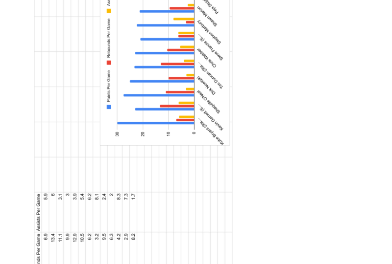We're going to use them here. I created this spreadsheet of the NBA All Stars from last season and the average points per game, rebounds per game, and assists per game. I'm going to use some of the functions in Google Sheets, the basic functions that you may use, especially if you are using I'm sorry, especially if you're working in Google Sheets often. Also you want to be able to use these if you have a large data. I'm sorry, if you have large data. Right here, I think it's only 20 players. But if you're working for a company and you have 2000 different people or numbers or whatever it is, it's going to be a lot easier if you know some functions and formulas. If I want to find the all star averages points per game, if I want to find the points per game of all the NBA Allstars, I'm going to go here. I'm going to use the function first. Insert, go to function, going to go to average, and I'm going to select all the points per game. Here, which is C three through C 22, hit Enter, and the average points per game of NBA all star from last year was 24.9 or 25 points. The cool thing about Google Sheets. I'm going to go to rebounds next and I'm going to start with my formula, equal. Google Sheets already believes that I want to get the average of D three through D 22, which will be the rebounds and it's correct. Because all this information here is correct, I will hit Enter. The average rebounds of an NBA all star from last year is 5.7. I'm going to do the same exact thing here. If I hit equal starting my formula, it's guessing that I want the average of E three through E 22, which is highlighted here and it's correct. Google Sheets is basically like a calculator. It's a smart calculator or smart calculator, but just like a calculator, it does all the calculations for you, but you have to tell it what to do. The great thing about Google Sheets and why I say it's a smarter calculator is because it'll guess as to what you want to do based on what you've done previously. Now if I want to find out the minimum points per game, what's the smallest number here? Because it's only 20, if I just scroll up and down a few times, I can tell what it is 18.5. But if I had a database of over 2000 different numbers, then this will come in handy. If I want to find the minimum number in regards to the points per game of last year, I go to the function here, then I highlight all these points per game. Or I select. Hit Enter, it's going to be 18.5. The exact opposite for MAX, go back up to insert function. MAX, going to select the points per game, hit Enter, it's going to be 32.7. Now, if I wanted to find out exactly what the total amount of points that scored on any given night in the NBA by the NBA All stars of last year, I will go to Insert function, some because it's going to add all these numbers together. I'm sorry. And it's 498 points. On any given night in the NBA last year, the All Stars scored 498 points. Now we got the basic formulas and functions out of the way. I also want to show you how to use cell references, but before I do that, if I go down here to sheet one, I can right click and I can rename. Here I'm just going to put MBA. If I click on Sheet two, I created something here, I'm going to right click rename and I'm going to type in I'm going to name it schools or school. All I created this worksheet, school supplies, and here I'm going to talk about cell references, relative and absolute. So here, let's say that the notebooks is a quantity of four. Each notebook is four, I'm sorry, $1.50. In order to find out what the total price is, I can type in a formula equal. Then again, Google Sheets is already guessing that I want to multiply these two numbers together. Google Sheets is right. Going to hit Enter. It's $6 for the total price. Now I can click on this seem sorry, the bottom right hand corner, this dot, I can click on that and I can drag this down. And it will do the multiplication on all these different numbers. This is what we call relative cell reference. If I open up the actual formula here, it went from B four multiplied by C four, to B five multiplied by C five, B six multiplied by C six, to B seven, multiplied by C seven, so on and so forth. But as you can see, it's relative. Because I did this, it believes I want to do this for everyone. It's relative cell reference. Now we're going to delete this information Be as of right now, let's actually type it in total. I want to type it in total. Here, and then I'm going to add these borders around. Oops. I'm going to add these borders around it. Here, if I type in some, it gets correct again. Now I'm going to delete this information. And obviously, total will come out to zero again. Okay, now because if you did take if you left the store and you've paid $325, that's cool, but you may have a problem at the door and the reason why is because you didn't pay any taxes. You may have an issue there. What we want to do is create a formula that includes the tax. Equal and we can do some or I can do it just the basic way I did it previously. I'm just so used to typing in some that I always type it in some. We take those numbers multiply it by C four, close parentheses, before, multiply it by C four, close parentheses. Then I want to multiply one plus the tax. Enter. Now you see that I multiplied it with the actual tax in there. That's the actual number now. Now what I'm going to do is I'm going to click on that cell. Bottom right hand corner, I'm going to drag it down because that's what I did previously so I can get this total number, correct? A got a problem. Whenever you see value, this number sign value exclamation mark, something's wrong. Why is it wrong? If you click on the cell, you can see the actual function or formula. Here, if I open this one up, it says B four multiplied by C four, multiplied by one plus D two. If I go to the next formula below it, B five, multiply it by C five, close parentheses, multiply it by one plus D three. This is D three. This is cell D three. It can't multiply some words. That's why you have this value issue. What we're going to do is we're going to delete this information. We're going to delete this information. I'm sorry, I just deleted this. I shouldn't deleted this part. All right. Now I'm going to go back into my cell and look at my formula. What I'm going to do now is instead of just D two, because remember, it's using the relative cell information or reference. It's going to keep going down. Remember how it went from D two, it went to D three. The next one was D four, D five. What I'm going to do here is I'm going to add in $1 sign in front of two. Why am I adding in $1 sign in front of two? Because it's still going to stay with the same column, but I want it to stay with the same row also. I'm going to put $1 sign in front of D two. You can put $1 sign in front of the D also, which is the column, but it's not necessary. You can. Now it's going to lock. If I put $1 sign in front of the D, it's going to lock this column and it's going to lock this row. But we already know the column is locked anyway, so I can hit Enter now. Now what I'm going to do, I'm going to drag this formula down and there are no errors here. Why? If I open this up, you see that it's still going to multiply this by this and then multiply one plus D two again right here. If I look at the next formula, it's the same thing, D two, because it's the only thing I wanted to multiply, sorry, it's the only cell that I wanted to stay on. That's an absolute cell reference. We got the relative where it also moves with the different rows, but if we want to absolute because we have to keep it here, we just add $1 sign in front of the row. You can add $1 sign in front of the column also, it's still going to get the same exact number. It's not going to change. That's some of the functions and formulas that's already in Google Sheets, or I should say the functions already there. The formulas, that's what you actually create and that's what you type in. Functions formula, you can use them interchangeably. Nine times out of ten is not going to get you in any type of trouble. 6. Charts and Visuals: Now that we have all this data and we've done different things with them, we want to work on charts and visuals. Now we're going to talk about creating a bar, line, and pipe chart, and then also how to customize these chart styles. So now you have this number or these numbers, I'm sorry, if you wanted to create a chart for them to make it a little bit more aesthetically pleasing, you can highlight the information or select the information that you want to be seen. Go to insert, then we're going to go to chart. It has suggested charts. The first chart that it created was a column chart and you can see all the names here. You can see the points per game, rebounds per game, assists per game. Here. Now, what you could do is go to Chart Styles. You can change the background color. You could change the border colors. Theme is default for the text or the font. What you can also do is, if you go to Chart and Access Titles, You can change the font size. You can do a lot of different things. You can customize it here. If you're looking to make it better on your eyes or the way that you're going to view it because it's all about you and your audience. If you know that you have to work with it every day, then you create it to the to the fashion that you want to create it because it's for your eyes. Creating a graph or chart for any of this stuff is based on what you want to see. Here, if I go back to the school supplies, going to hit control. I'm going to take the items and the total price of the items. Going to go to insert? This is selected over here, sorry, for some reason. Okay. Going to go to insert, going to go to chart. As of right now, let me make it a little bit smaller so we can see. Here it is. It has the notebooks, pencils, binders, eraser, divider tabs, calculators, headphones, how much it costs, total. How much each item costs in total. Here it is. Now, what we can do, we can change this chart to a bar chart. You could change it to a pie chart, but we know that pie charts are a little different. So what it's showing is it's showing by percentages. So you can see the percentage in regards to the amount of money that's spent or the total amount for each item. So here are your charts. Again, you create it how you want to create it. What's going to be more aesthetically pleasing to you and your audience? So if you're creating this for students, you're creating this for coworkers, you're creating this for family member or friends, you have to think about what's going to be more aesthetically pleasing to them. If it's just for you, what's going to be more aesthetically pleasing for you? Because you have to work with these things. But that's how you create the different charts. 7. Conclusion: We have now come to the end of the Google Sheets Essentials course and I want to thank everyone for selecting this course. I want to also congratulate you on completing this course. In conclusion, we went over navigating the workbook, data entry, and formatting, basic formulas and functions, and charts and visuals.