Transcripts
1. Basics first intro: Do you want to learn
axon from scratch or do you already know
your way around Excel? I want to set the
fundamentals right? Or maybe you look for
tips and tricks to become more efficient
in working with Excel. Then there's actual
bootcamp is for you. Hi, I am bus and I'm a trainer
and consultant for Excel, Power, BI, and Tableau. I run my own company. They are training IO.
I'm also a YouTuber. I've built this complete
online actual training to help you master Excel and the quickest
way without wasting time learning things that
you want to use in practice. This training is
the first part of a complete axle boot
camp that takes you from beginner to a very
professional user. In this part, you will learn all the basics you need to get started before diving into
different focus topics. So let's get right to it.
2. Shortcuts for selecting data and moving around the workbook: When you work in
Excel, it's very important that you have a
good understanding of all of the basics and
fundamentals before you move into the more intermediate
and advanced topics. Now I've seen a lot
of people that work already for quite
some time with Excel, but still don't know many of
the basic functionalities. So in this section we're going
to have a look at all of these fundamental things
that you really need to know when you start
working with axial, like formatting, doing transformations to your
sheets or columns and rows, and working more efficiently
using shortcuts. Let's get started. The actual workbook that we're going to use for
this section you find in the first
folder, basics first. So let's go there and
open the Excel workbook. And we're going to start off
on the sheet that's called example one, hotel booking info, where we have a dataset
about the bookings for different hotels with data on the booking day
to check in there, how many people came
along, they stayed, etc. For most of the transformations that you're going to
do an excellent you first have to
select the data and then apply the transformations
do the selected data. For example, if you want
to adjust the formatting, you first have to
select the cells and then apply the formatting. Or you want to
summarize the data with a formula that uses maybe the sum or the
average function. Then you need to select
the range of which you want to take the
sum or the average. Now, because this is something
that you do all the time, you want to do it in
the most efficient way. And this is where keyboard
shortcuts command. And you might think, oh, I'm just starting off with axial, why they already come
with keyboard shortcuts, because it makes
your life so much easier and it can work so
much more efficiently. I think it's something
that you need to get used to store it away
from the beginning. So let's have a look
how we can select the data over here in
the most efficient way. Well, one option that we
have is to use the mouse. We could go over here to B3 and then scroll all the
way to the right, and then all the way down. And with the scrolling,
we'll go down and down and down until I reached
the end of the dataset. However, if you
have a big dataset, this could take
quite a long time instead of doing it like this. But the mask, we're
going to look at the alternative
using the keyboard. Now, we're gonna go
back to the top. Here with the arrow keys. We're going to select cell B3. Now together with
the Control key and the arrow to the right, you see we jumped
to the cell W3, which is the last cell
that contains some data. And if you do this once more, then we jumped to the very
last column in the worksheet. Now if you do the opposite,
so control to the left, then we are back to W3 wages than the first cell
with data that it finds. And if I do it again, once more control to the left, then we back in cell B3 because to the left of
B3, there's nothing. Now of course, this
also works vertically. If we select B30 again
and then control down than we are in the
very last cell where we have some data. Because right below it
you say There's nothing. If I do this once more. So control down,
then it brings us to the very last row in the
worksheet and control up. Then we are back
in cell B, 5,003. And once more than we
were back in cell B3. So this is how we can jump very quickly from one side
to the other side. Usually we don't just want
to jump to the other side. We want to select
the data in between. This is where we also have
to hold the Shift key. So if we select b3 again, and now we hold control
and the shift key, and then we press the
arrow to the right. Then you see we again go to the cell W free but select
everything in between. Now we can also go down. So hold Control Shift
and the arrow key down. And we go all the way to
the bottom of a dataset. So we have the whole
dataset selected. Now, if we want to make an adjustment than simply
hold the Shift key. And then with alkenes
we can go to the left or we can go up a little bit to adjust the selected manage. Now let me go back
to the top again, control up and to the left. So to select data in
the most efficient way, you can use the arrow keys in combination with the
Control and Shift key. Now if you already know that you want to select
the whole dataset, then there's also another
alternative that you probably want to know
and that is control a. If we select any cell
inside of your dataset, and then you do control a, they see it also select
the whole dataset. However, control shift
is still very useful if you don't want to select
the whole dataset, but just parts of it. Another thing that you will be doing all the time when you work in a workbook is to jump
between different sheets. Now of course, you
can use the mouse to click on the sheet
you want to go to. However, we can also
use the keyboard, which is maybe a little
bit more efficient. Go to the page that's to the right hand side
of the current one, the Control key and then
base down if we want to go to the beach that's to
the left of the current one, then all the control
key page up. Alright, so now you already
know a few shortcuts. Now if you want to
have a full overview of all the shortcuts there, I included a PDF that
you can print out. Now, don't learn them by heart because that's
completely useless. Now, only learn
those shortcuts for transformations that you find yourself doing all the time, like during the training,
I will highlight those shortcuts that I think
you really need to know. And of course tried to use
them as much as possible. Then the next section
we're going to create a short summary table in which we are going to talk
about how to enter text values and needs.
3. What you need to know about text, values, and dates: In this section, we're going
to create the start for the summary overview that you find on the sheet and result. Now, to create a summary
overview like this, we, of course, need to enter some
text, values, and dates. And that's the main focus point. Now, we're going to start
off on a new sheet. Now, to insert a new sheet, we can either click there on the plus icon in the
bottom right corner, or you just right
click on one of the sheets and then
click on Insert. Now, we want to have a
worksheet, and let's click on. Now, if you want to
zoom in a little bit, we have the Zoom button here
in the bottom right corner, where we can zoom in and out. And let's start by giving
an overview a title. So here we're going
to answer some data. About the booking info. So I'm going to call
this one booking info, hotel one and two. And then using the RO Keys, we go to sell eight three, and here we can type
in the headers. Maybe the hotel, and then with the ro key to the right,
go to the next one. And here we want to
have the hotel ID. And here we can have the
booking date. All right. Now, there are a few more,
which we can add a bit later. Now, for the hotel, let's
just type in here hotel. One. And then here
for the hotel ID. Let's say we're going to have in the summary overview
just five bouquets, so I can type in one, two, three, four, five. Now, at this point, you should already notice one
big difference between those cells in which we have the values and those
cells when we have text. By default, you see that the values pop up on the
right hand side of the cells. So they align to the
right hand side. However, for the text, it aligns to the left hand side. This becomes clearer when I make this column a
little bit wider, which I can do by placing
the cursor in between the heaters for column B and C. You see the
cursor changes. And now I click and drag that column a little
bit more to the right. And then you can
clearly see that the values are
aligned to the right, and text is aligned to
the left hand side. Now this is something that
you always want to check before you start
analyzing your data, especially when you
have a new data set, where you have values and dates, that can quickly go wrong. Now, let me give you an example. Let's say we would not
have whole numbers, but we would have
decimal numbers. So, for example, 1.5. You see 1.5 pops up on
the right hand side, which is where it should
be because it's a value. However, let's say we would
have data from a region, where as a decimal separated, a comma would be used, and
I start using that data and Excel didn't interpret it in the right way, then
this could happen. One comma five. And you see it pops up on
the left hand side. It recognizes it as text. So therefore, always
double check this. Now, After you check this, then of course, you could
change the alignment. You will see that here
under the home tab that we have different
alignment options. For example, we can say
aligned to the left. However, by default, it's always aligned to
the right in side. Now let's remove
these values again, which we can do by selecting
before and then hold control shift down to select all of the values and
then press delete. Okay, so the values are gone. Now, you saw before when
I entered the values, I did it manually, one by one. So one, two, three, four, five. Now, for five values,
that's not a big deal. However, what if
we would have 100? You don't want to
do this 100 times. Now there are different, more efficient ways in which
we can fill up the series. Now, as an alternative, we can also use the fill series option, which you can do
by first selecting the cell with the
one, then go to home. And then a little bit right from the middle, there we have fill. Now, we want to have a series. So we go for a series. We want to fill it down,
so in the columns. And here we want to go
from one, two, five. And the type, you see, we have also this option
for the dates, and we can have also
growth if we want to. But here we keep it simple. We just go for linear. Okay. Good. And we have
our series with 125. Okay, so far, we entered
text, we entered values. We used the series
functionality. But what we didn't do
yet is entered date. So let's go here to sell
C four and enter a date. Now, in the end result, is the first booking
date, we have 22 January. 21. So let's type this in. So I'm going to enter 22. And here we have an
option for a dot or four slash or a minus
sign, whatever you like. So 22nd of January, so one. And as the last
argument, the year 2022. Okay? Now, here,
I'm going to make this column and get a little bit wider, so just like this. Okay. And you see it
shows on the right inside of the cell,
which means, well, just like a value, it
bumps up on the right, because actually a date, is stored as a value. Now, to show you this, we
can change the formatting. Now, the formatting you find under the home tap
here in the middle, you see here we have
different formatting options. And instead of
formatting it as a date, we could choose either
general or number. Let's go for general. You see the underlying number as
which the date is stored. 44,583. What does that mean? Well, that is the number
of days that we are away from 1 January 1,900. So if I would have
typed in here, 01011900, And then
change the formatting. Two, general. You see?
That is number one. But what if you have
dates before the 1900s? Well, then L cannot really work with
those dates as dates. But of course, for most people, you have dates that
are after the 1900s. Now let's do what we just did, which we can do by
going to the home tab, and then here on
the left hand side, there you have the undo
button and the redo button. Okay, so here also
the shortcuts. Control Z, Control Y. Try to remember those. So I'm going to undo it, Control Z. And let's do this once more and once more until
I get my date back. Now, it might be that you
have done exactly the same, but your date looks a
little bit different or your date pops up
on the left side. Well, that has to do with
your regional settings that you're using in windows. If you want to change or check what regional settings
you're using, you just go here right next to the windows button,
type in region. And you see here we
have region settings. A new window pops
up. And from here, we can say what region we
are using for the format and make individual changes to how the short date and long
date should look like. But also here in the
additional settings, we can change what our decimal separator
should be. All right. Now, here, I'm just going to
leave everything as it is, and we turn to Excel. All right. So if you're in the US, just type it in
in the US format. So first the month, then the days, and
then the years. Okay, but just double
check that when you do it, that the date pops up
on the right hand side, because Exel should store it
as the values and values, they align to the
right hand side. Now, let's say we want
to create a series where we just increase that
booking date by one day. Then we can just take what
we filled out over here, go to the bottom right corner. You see the cursor changes,
to a little cross, and then we can drag it down
and fills up the series. This would be one option. Now, if you don't
want this series, then you could also click on the plus icon and say that you only want to copy this sale. Okay. Now, let me undo this
and go back to C four. Alternatively, we
could also go to the home type again
and then fill, ten series, and then
here we can say that we want to have
it columns type. Now it's date, and here we
want to have date unit day. And also interesting is that here you have different
options like Mon V here, and you have to
say what the step value is and the stop value. Now, the stop value, either you put in the number that
corresponds to a certain date, or you could also just
type in the dates, huh? So over here, we want to
have five days in the end. So I type into 26th
of January 22. Click Okay. And you see, there we have our
series of dates. Now, if you want to
practice a little bit, then also add the other
columns and all of the data. Just go back and forth
between the end result, and the result of this part should look like this
over here. Alright. In the next section,
we're going to have a look at different options and transformations that we can do for sheets, rows, and columns.
4. So what options do we have for sheets, columns & rows, and cells: So now we have the
basic structure of this summary overview
that we want to create an excellent
if you want to have a look at the options
for certain objects, whether that is a cell
or range of sounds, rather that is column or row. Or maybe she'd just right-click on the object for which you
want to change the options, and it will give you an
overview of what is possible. Now as an example, let's see what options we
have for a sheet. Now, here we have she'd won the sheet that we are
currently working on. And I right-click on it, and you will see we have the
option to insert a new one, delete the current
one, rename it. Now let's do this. Let's rename the sheet, and
let's call this one example. Now let's right-click on
the same sheet again. And let's have a look at some
of the other options so we can move or copy the current
sheet somewhere else. Over here. This can be within the workbook. And here we can also
choose a new workbook. So if you want to just copy
it over to a new workbook, you would say no book. Create a copy. Click. Okay. And now I create a new AKS, a workbook with that same sheet. Now let's go back. So I minimize this new workbook. Now let's right-click on
that same sheet again. And here you see we
have dark color. If you want to assign a
certain color to cheat, then you can do that over here, that this can be
very helpful if you want to keep everything nicely organized and assign a
certain meaning to a color. Alright, now, for this example,
I'll just go for blue. And here at the bottom then we can also hide or unhide sheets. Now if you hide it, then you see it disappears. However, we can
always bring it back by right-clicking on one
of the other sheets now, so if I right-click
on any sheet, doesn't matter which one, then I can bring it back over here. Example and click. Okay. And now it's back. Now just like we do
transformations on sheets, we can also do transformations on columns or rows and cells. Alright, now let's first have a look how it works
then forgotten. So if we want to
adjust the column, we already have seen
before that we could left-click on the
column header and then go in-between the column headers and then the cursor changes and we can increase or decrease
the width just like this. Now if you make it too small, then you will see
hashtag pound symbols instead of the actual values. Now that just means
the values don't fit. So you have to make it
a little bit wider. So we can then just drag it to the right
so that it fits again. Or alternatively, we can do this also for
multiple columns. So if I select all
of the columns and then adjust the width and the same width gets applied
to all of these columns. Now, if you want to do
this automatically, then let's say it is like
this and we want to alter, adjust the width of the columns. Then you go Also in-between one of the columns and
just double-click. And then it makes it as
wide as it needs to be to fit in the content that's
inside of that color. All right, now,
just like before, we could also right-click
on one of the colonizers. So let's say I take
this one over here, right-click on the
column header. And here you see
we can either got a copy that column and then
paste it somewhere else. Or we can insert a new column, delete the column
clearly contents. Now, I think this is quite self-explanatory
and what it does. But the one that's kind of interesting is also
here at the bottom, where we can then also
hide it or neither column. So if we hide it, you see
we are hiding that column. We want to bring it back. Then we just select the
columns right next to it. And then right-click on calmer, unhide it, and that
brings it back. Now, the one that gets to be tricky is the very first one, because there's no column
to the left of it. So if you do this for column a and hide it, you
see it's hidden. And now you will have
to select column B and just drag your mouse and
a little bit to the left. Alright, and then
right-click and unhide. And this way you can also
add bring back colony. Now hiding an annealing
is no production, okay, So you can always bring back that column by right-clicking
on the column or the sheet. However, what often happens, especially when you
have hidden sheets, is that people
forget about it and then send that maybe outside
of the organization. And this way, you might share data that you were not
supposed to share. Always watch out before you send something
to somebody else. Double-check in your
actual workbook. Artists steal it in sheets and
maybe take them out first, especially when you
get it from mechanic, then you might not be
even aware that there are hidden sheets and that
there are hidden Collins. So always double-check this
before you send it out. And of course, also when
you get an actual workbook, then one of the first things
that I personally do is jack or the hidden sheets because you never
know what you find. The next section
we're going to have a look at different clever task. So how can we bring over
data that we already have in a different sheet or
a different workbooks to the current sheet.
5. Copy pasting data - clipboard tasks: So let's have a look at
different clipboard tasks. How can we bring data over from one sheet or another
workbook to the current one. Now, for this, we're
going to work with the same example that
we built before. So here we have our data. We have the main
structure set up four, only Hotel one, but we also
need the data for Hotel two. And you might have this data
already somewhere else. So here in our case, we have it on the
end result sheet. Now we can click on it, but try to use the
shortcut keys. So with control and then
page up or page down, we can go to the
end result page. Now, From here, I would like to have the
data for Hotel two. Now, you see, I'm using OKs. I'm going to go all the way to the left where
we have hotel two, control shift to the right, and here we have
all of the cells selected that I
want to bring over. Now, here to copy it, we can do either the following, we go to the home tab, and then from here, cut a copy. Now, what is the difference
between cut and copy? If we copy, then the
data stays here. However, if we do cut, then it will
disappear from here. Okay? Now, You see
when I hover over it, there it also gives
you the shortcuts, which is actually also very helpful in this case and one
that you want to remember. So for cut, it's control X, and for copy, it's control
C. Now, alternatively, you can also always just right click on the object
that you're working with, which is in this case, a range. And then right click. And
then you see over here, we have cut and we have copy. Now, Let's go for copy
or Control C. Now, when you do this, then you see a dotted line going around. That means at the
moment it's copied, and then we can go to the sheet where we want to have this data using the shortcuts control
in that page up or page down. And here we want to
have it in A nine. This is the top left self of
where we want to have it. And then we have
to click on paste, either here and the home tab or right click and then paste, and you see we have
different options or shortcut Control
V. And actually, this is a transformation that you really want to
know the shortcut of. Control C, Control V. You will be doing
it all the time. Control C to copy,
Control V to paste. If you want to cut, control x, and then control V
to paste. All right. So let's do control V. Now here, you see everything was copied, also the formatting
of the values. Okay, so that you don't
have to redo it again. However, this might be a
good thing or a bad thing. If you only want to have
the values, let's say, then we can click you
on the control button that is there in the bottom right corner,
so the baste option. Now, if you want to do
it with the keyboard, you can also actually
hit control, and you see all of the options. Now, over here, you
see we can paste only the formulas or
only the formatting or only the values. That's so you're flexible. Okay. Now, let's say we only
want to have the values. Let's go for the V option,
so that's this one. Values. All right, see,
also for the dates, we then only have
the numbers, okay? The numbers that underlie
basically these dates. Now, you see, we have
one column extra. That's because over
here in the end result, I have a check out date. And here in the example
that we bill before, we only have the booking
date and check in date. Okay. Now, either we insert over here a
little bit of space and then find the data
for the checkout date or we get rid of that column. Also here, select the cells that you want to
get rid of that you want to do a transformation
to, right click, delete. And here we want to shift
the cells to the left. Okay. So now, the next
thing that I want to have is the same formatting applied
to the bottom section. Now, here we can select those cells from which we
want to copy the formatting, control C to copy,
and then over here, we can only paste the
formatating this option here. Okay. Now, I want to have Hotel two also here
for the other cells. So I just drag it down. However, you see it automatically
increases the number. So I click here on
the control box and choose copy cells. All right. So now that we have
all of the data that we need for a
summary overview, let's make it a little bit prettier and adjust
the formatting.
6. Making everything pretty with formatting: So we have all of
the data n. However, it doesn't look so pretty yet. So how can we make it
look just a bit nicer? And how can we, for example, adjust the formatting
for the values for the day or maybe add
a little bit of color. And maybe we will also
want to get rid of these grid lines that you
see there in the background. Now, this formatting
options we're going to talk about
in this section. Now let's start by having
a look at the end result. What do we want it to look like? Now, let's say this is the formatting that
we want to go for. Now here at the top, you see I made the title a little bit bigger
in a different font color. And we added over here a different background color for the headers and a different
font color as well. Then you see we have some
grid lines in the back. We have merged cells here
on the left-hand side. And space around it is just
nice, clean and white. Okay, Let's go now to
our current sheet. So I go back here. Let's start by updating the
formatting for the title. So I select here cell A1. And here we can make the
font a little bit bigger. And we can also
choose a different form if you like to do so. Alright, so let's go for
a bigger font, maybe 18. And then let's give
it a different color. Let's go for blue. Now here I would like to
have it in the middle. One option is to select the
cells that you want to merge. And then here at the top
you'll find merge and center. So different options in
which we can merging cells. So if we click on
Merge and Center, it becomes one big cell. However, try to avoid
merging as much as possible because it can lead to traumas later down the road. So if you can avoid merging
this case, we actually can. If I undo this,
click on it again. We can also right-click on the object that we want
to see two options, for. This case, a range of cells. Now, we want to
format the cells. Now, click on it. If you want to know the
shortcut is Control one. So maybe another shortcut
that you want to learn. Over here, select the cells, control one formatting
options pop up. And from here we can choose
a different alignment. Here we have
horizontal alignment and we want to center
across the selection. Click on Okay, and this way we don't have to
merge the cells, but it still shows at the
very center of our cells. Okay, now, perfect,
So we have the title. The next thing that I want to do is make these grid
lines disappear. Not what I see a
lot is that people select the whole sheet. So every single
cell on the sheet, and then going into home and apply in different
background color. But if you do that, they do it for all of the
cells in the sheet, which you probably don't want to do it because there
are million rows, about 16 thousand columns. What that is a lot
of cells, right? So instead of that, let
me undo this Control Z. And now we go over here to Page Layout and turn
the grid lines off. Or alternatively, you
can also go to View. And from here, you
can also say that you don't want to show
the grid lines, okay? Now, in this way, you can
always bring it back and you don't have to apply different background color
for all of the cells. Now, we want to have a different background
color here for the others. So that's like the
others go to Home. And then here we can adjust
the background color. Let's maybe go for blue as well. Now, also here, alternatively, you could also have
done again control one. Go here to the fill options
and choose a different color. Now, these options that you see here correspond to the options
that you see at the top. So most of these options you find either here
under the Home tab, here under the
formatting cells window. And when you right-click on the cells and go to
Format Cells options. Now let's click on Okay, now we want to have a
different font color. So also here, either control
law, change it there, or directly here on the Home
tab and maybe go for right. Okay. Now next thing that
I would like to do is I would like to
have some grid lines, some grid lines
in-between the rows. Now, here, select the cells to which you want to apply and grid lines either going into the top, go for one of these options
are CO2, more borders, which then brings you again to that same format cells when
asked where we were before. Now here we want
to add a border. Then here on the style you can
choose the border diapers. So maybe we want to have
these dotted lines. We want to have
them in light gray. We want to have them in-between. Click Okay, you see we have
this dotted lines in-between. We'll also want to
add a border line around a summary overview. Select the summary overview, either control one
borders or we go here. And maybe you want to have an outside border
just like this. Maybe you also want to have a borderline
in-between hotel one. And what they'll do is do this. And then we have also a thicker line
in-between right now. Okay? Now let's insert over
here new columns. So right-click and
column a, insert. And here we can adjust
the width of the columns. So let's do that for
all of the columns. If you want to have equal f, just go in-between
the column headers, then adjust one of
the columns and you see it gets applied to all
of the selected chords. Alright? So just play around with
it until you're happy. Now maybe here for
the beginning ones that's made these two
a little bit smaller, but they don't take
that much space. Perfect. And what about the
number formatting? Because here we have values
where I actually want to show a currency symbol or maybe I also want to have
decimal places here. Well, this has also
formatting, but Number Format. Now also here two options. Either we change it
here under the Home tab and then go here to number,
number, formatting. And here we see all
the different options when you click on the drop-down. And also here we have
more number formats. Or we do again control one
and then go here to number. And here you see,
we also have all of these different options
to choose from. This case, we could go for number or maybe
currency or accounting. Now, in this case I do want
to have currency symbol. Choose the currency
symbol that you like. So maybe over here, Let's go for the Euro symbol over here.
I just have to look. Euro symbol, German, Germany, where am at the moment. And then adjust
the decimal places we have assembled behind. Perfect to control the space at the top a little bit more, what you could do is maybe also insert an extra
reward at the top. And now the last part
that we still need to set up page layout, something that's
often overlooked. But it's very quick to setup. However, can be very
frustrating when somebody doesn't do it and 90% of
the people don't do it. Which means that if
you click on print, it prints out in the wrong way, which can be very
frustrating and always happens at
the wrong times. So that's going to
be the next topic.
7. Getting everything ready for printing: Now we're almost at the end, we have a summary table. The formatting is setup. However, this very last
step is very important. Page layout makes sure that when somebody
clicks on print, it prints out in
the correct way. And this is something that
too many people skip, but it's very quick to setup. So make sure that from now on, you're always set
up the page layout. Now, where can you set
it up? Two options. Either you go here
to Page Layout and then you find
things like margin. How much space you want
to have around the page. Then we have
orientation, portrait, landscape, size, print area. And this is the most important and usually
my starting point, what part of the sheet
do I want to print? So let's start there. You can either select what
you want to print from here, go to Print Area,
set the print area. Now, this is one option. Now another option is
to actually go here to the bottom right corner where we have the zoom buttons
are right next to it. We have these three buttons. The first one is what we are currently looking
at, the current view. But the last one
is the one where I switched to when I want
to set up my page layout. Let's zoom in. Now here you see this
blue border lines, and it's blue border lines
indicate the print area. We can adjust it so
that only this part gets printed out and
everything fits on one page. If we wanted to have
an additional page, we can add breaks into it. So make sure that everything
that you want to be printed out is within
the print area. And once this is setup, you can also go to
the middle part. When you also see the border. The border is around that. So basically the margins and extra stuff that you're
going to put in the headers. Alright? Now, after this is done, I just return to
the normal view. If you want to get
a full overview of all of the options
that are there, I usually would go
down to Page Layout. And then here click on
the little arrow in the bottom right
corner, Page Setup. Now here you see we can
set up the page just like we could do also directly
from the ribbon. Here we have margins. Add a footer if you want to have a header or footer sheath. And the one that is most useful, I think, is the Rows
to repeat at the top. If you have a large
dataset and you print it out and it prints out of
done different pages. Now let's say that
you have headers. Well, you don't want
to go back and forth between the different
pages to say, okay, if third column
means this field, okay? Instead of that,
you might want to repeat that part, okay, So you can just click on the button to
select the rows you want to repeat on every single
page and click on, Okay. Okay. In this case is not relevant because everything is
just on one sheet, but if you have multiple pages than this becomes very relevant. So this brings us to the
end of the first section. We covered things
like how to enter text values and dates and what
you have to watch out for. We talked about different
clipboard tasks, how to bring over data from one sheet or workbook
to the current one. We talked about how to do transformations to
sheets, columns, rows, and also to individual cells, and to get the formatting exactly the way that
we want it to be, I hope that you're excited
to go to the next part. We will talk about
formulas and functions to add additional insights
to our summary overview.
 Bas Dohmen, Founder + YouTuber