Excel VLookup Function: Learn The VLookup Formula With Examples

1. Introduction: Hi, I'm Gary, a data analyst and the founders skill quest. And I'm really excited to welcome you to my Microsoft Excel VLookup masterclass exclusively on Skillshare. Now in this class we're going to learn all about the VLookup function, which is one of the most valuable and powerful real-world Excel skills to have. And that's why I designed a whole course around it. Now, during this class, you're not just going to learn how to do or be looked up, but you're going to learn the why behind it. Next, we'll explore multiple different examples that you'll be able to try on your own throughout the course. We're also going to look at the top common issues that can occur and also how to avoid them. And lastly, we're going to have a challenging class project at the end so you can test out all of your new techniques that you learned in this class. Now I designed this class for the absolute beginner who wants to learn the VLookup function in an easy to follow and engaging way. Now my goal with this class is to take you from absolute beginner level to approach. Or you'll have the confidence when you leave to be able to apply those techniques that you learned here to the real-world, whether it's your job or your business. So if you're ready to up your Excel skills and learn all about the lookups. I welcome you to join my Microsoft Excel. You look up skilled west. I'll see you there. 2. Getting Prepared For This Class: Now I do want to share a few tips really quick before we jump in. First tip, if possible, I would suggest using headphones so you can hear the audio clearly while avoiding any distractions. Or if you prefer not to, I would just suggest simply trying to be in a quiet location. Next, if you feel a certain lesson wasn't completely absorbed, I would suggest re-watching the lesson again and then trying yourself on the example sheets I provide. That way you'll be a 100% ready to go and move forward to the next lesson. Next, I would just make sure you're at a computer that has Microsoft Excel 2013 or higher. That way you are able to follow along and try the examples that I'll be providing, as well as complete the project at the end of this course. Next, I would suggest that Justin, your volume, your video speed, and your video quality if needed. And you can do this by just hovering over the video screen at the bottom here. And your Skillshare video bar will pop up and you'll see all the settings within that bar that you can adjust. And then lastly, I would suggest trying to block off enough time needed to complete all of the lessons you'd like to finish today. 3. Why The VLookup Is Important: Alright, so now that we're prepared, Let's start our quest. The VLookup function, in my opinion, is probably the most important Excel formula to know if you have a job and where you use Excel. It's not too complicated at all. Once you understand how it works, the same time, it's just an extremely useful and powerful tool. I remember many years ago prior to me being a data analyst, I was on a job interview and I was asked if I had experienced in Excel, which I said yes because I did. But then I was asked if I knew how to do a VLookup. And I remember the time I heard of it, but I didn't really know how to use it or what it was for. I was truthful and I just said, I don't needlessly, I did not get that position at the time, but that experience actually gave me the desire to not only want to understand the lookup was and why it was so important, but also to become as advanced as possible in all aspects of Excel, which ultimately led me to becoming one of the top analysts within my company. So why is it important? Why do a lot of job interviewers ask this specific question? Well, if you work in Excel every day, there's a good chance you work with different spreadsheets that contain different data within them. And some of those spreadsheets may have data that's related to the data on other spreadsheets. And a lot of the times you may find yourself needing to merge data from different spreadsheets into one spreadsheet, right? And then once you have it in one table or one spreadsheet, you can analyze it from there, right? Maybe you need to throw it in a pivot table or make an awesome chart like you see right here that I made, right? So understanding how to do a VLookup, it's just a very important skill to any job position that involves the use of Microsoft Excel. 4. How The Vlookup Function Works: So the VLookup formula, I think, is one of those formulas that can be difficult to perhaps understand at first. So I'd like to start with an example completely unrelated to Excel. We actually perform VLookups outside of Excel in many real life situations. For example, let's say you go out to eat. Let's say you walk into a restaurant, right? That makes subs. And you really want Italian sub. So you know, you want to tie in sub, but what you really want to know is the price for a large Italian sub. Alright, what's the price? Well, in most cases that would require you to actually do a VLookup in your head. First, what you're going to do here, when you're looking at the menu, you're going to look in the item column until you find the Italian sub. Is that the item that you want? Once you have found it? You've linked the item in your head that you want to, the item that is on the menu. So you've got that link. Okay, Now, the next step here is you're going to move your eyes over to the right until you get to the column that has the price of the large Italian sub. And once you find it, you're all set right now you know the price. And you've basically brought that price over from the menu to your head. And you know what the price of the large Italian syllabus. And really that's, that's essentially what a VLookup does. 5. L1: Vlookup Into One Cell: Alright, now that you understand how the VLookup function works, you're ready to move out to less than one. Now, in lesson one, what we're going to do, we're going to learn how to bring in one value into a cell. So in this example, we have a worksheet that will give us the account name in cell C6 based on the account number that we enter in cell C4. So every time we enter into an account number in cell C4, we want the account name that's in cell C6 to automatically update. Now, to do that, we're going to have to write a VLOOKUP. So step one, we're gonna tell VLookup to look for this account number that we'd typed out right here, and that's in cell C, C4. Step two. Next, we want to find that value in this first column of this whole range that we highlighted. Step three, if it does find that account number and we have a match, we want Excel to bring over the account name. And it's going to be in the third column over from our matching column, which is our starting column, right? So we would enter in a three. And then the last step, we're going to enter in false or we're going to choose false. And that way, it's going to look for the exact account number that we typed out. We want to make sure it matches it exactly. So that way the account name that we bring back is going to be the right one. So take a good look at this formula we have here. Okay, Pause if you need to. Alright, so let's see if we found a match. Okay, so we can see that it found a match, match the account numbers. And then after it found that match, we told the VLookup to bring over whatever value is in the third column over from our match. And in this example it's Hanford. So we brought over Hanford. So now what we're going to do, I'm going to jump into Excel. I'm going to do this exact example live for you. Alright, so the first thing we're gonna do is enter in an account number in cell C4. So I'm gonna double-click in there. And we're going to type out in account number. The account number I enter just for this example is for target, right? So next, we need, our goal is to bring in the account name into cell C6 based on the account number that it's related to, right? So in this example, we would want to target to populate right there. So we're going to start typing out our v lookup formula. So I'm going to double-click in this cell. And I'm going to type equals V L. And I'm going to press the Tab key. Now, I could type out the whole equals b look-up and spell it out. But you don't need to because as soon as you type VL, you'll see that V lookup, the function name populates right below. And then you can just simply click Tab. It does it for you, and then it opens up a parentheses, right? So now we're ready for step one. Lookup value. What do we want to look up? Well, we want to look up the account number. So I'm just going to click in cell C4 because that's where the account number is. Alright. I'm going to press comma. And now next step. Where do we want to look for that account number? Okay, where's the table array that contains the account number? Well, I can see it's in, it's in column E. So I'm going to start there. And now I need to ask myself, okay, Well, I found the column that I want to try to find a match with. I know that my account number, I want to look for it in this column, but if it does find a match, okay, what do I want to bring over? If I wanted to simply bring over the account number, I could just stay right here, but I don't want to bring over the account number. I want to bring over the account name. So I'm just going to hold my left-click down and highlight all columns until I get to the account name column. And if you look really closely at the top right, you can see Excel actually shows you how many columns you're highlighting. So for example, right here are starting column, right where we want to try to find a match. It's number one, it says One C. And if I keep going all the way to the account name column, it says three C. So I'm already prepared for my next step because I know exactly how many columns are over. I need to be to get to the account name. So I'm going to stop there. Press comma. And now step three. Okay, how many columns over? Well, we already said that it's three. We saw that. So we're going to type three comma. And then the last step, we are going to select false for exact match. So I'm just going to use my down arrow and then press tab. And then I'm just going to close my formula with a close parentheses and then press Enter. And it worked. So now let's, let's try another account number, see if it works. So I'm going to do shows. And it worked, right. We have shows in here and it populated. Let's do the account number for Walmart. And we're good. Alright, so that's one way to do a VLookup. Now I'm going to show you another way we could have done this VLookup. I'm going to clear out this formula completely. And we're going to double-click in here and do it again. So I'm going to type equals VL, and I'm going to press Tab my lookup value. Again, I'm going to click C4 and press comma. So, so far we haven't changed anything. But for the second step, instead of me highlighting the entire column or all three columns completely, I'm gonna do it a little different. I'm just going to select the range that contains the data within the columns that I want to look up. So in this example, we're just going to select E4 to G4. And now the rest of the steps are exactly the same. So that was the only difference, right? Comma. We'll do three for the third column. Again, we'll do an exact match. Press Tab, close your parentheses, and you're done. Now, if you are going to use a range though, it is always best practice to lock the range in place. In this example. In particular, we don't have to lock it only because we're only looking at cell C6. So that range that we just highlighted is never going to change. However, we were working within a spreadsheet that had VLookups that we're going down a column, right? Let's say we wanted to bring in VLookups for account numbers all all the way down, right? If we did that, the range would actually change. If you look closely at the formula, see how it pushed down. And then each time it pushes down, right? So because of that, best practice is to always lock your ranges up to weight, the weight and lock it up. As soon as you go to step two and you select your range, you just going to press F4 on the keyboard to lock it in place. And then I'm going to, again, we'll go third column, exact match and we close it. Now you may be thinking, well, why would I do that? Why do I want to waste my time having to highlight an entire range of data and then lock it up. And honestly, I, I agree. I, 99% of the time, I just highlight the columns themselves. It saves me time, and it works perfectly. The only thing you need to be aware of though, if you do it that way, is you need to make sure that the columns that you're referencing are clean. And when I say clean it mean, I mean from top to bottom, they only contain the data that you want to look up and bring back in. Okay, so for example, let's say this was a spreadsheet that was not very clean or was the spreadsheet that had multiple lookups in it. And we had this random data underneath. That's a situation where highlighting the entire column would not be a good decision. So to summarize it, anytime the columns are clean and don't have unrelated data, we can just go column the column. However, if there is unrelated data and, or you just want to focus on a particular group of data within the columns themselves. That is, when you would use a range and you would lock it up. Again. We will explore this a little deeper in lesson two. Alright, so at this time I would encourage you to go to your resource section of this Skillshare course and open up the lesson one Excel workbook. You go to lesson one tab, and then you can practice. You can go to cell C6, double-click in there and practice writing a VLookup. If you get stuck, you can ofcourse rewatch portions of this lesson or you can even go over to this lesson one Completed tab, and then click in cell C6 and it'll show the formula for you. Alright, so good luck with that, and I will see you in lesson two. 6. L2: Vlookup Into A Column: Alright, great job completing Lesson one. Now we're moving on to lesson to lesson two. We're going to learn how to bring in lookup values down an entire column all at once. So for example, we want to bring in the product prices for these five products that we have here on the left-hand side. And we're going to use the ID as our link, right, to bring that product, those product prices over. Because we know the ID exists in both tables as we can see. So let's review the steps to do this. So step one, we're going to look at the product ID that's in cell B3. Step two, we're gonna go search for that product ID in this other column. So this column F, That's our starting column for our table array. Now we're going to highlight all columns of this table array until we get to the product price. Step three, we need to know which column the product prices in that we want to bring over. Well, we know our starting column is always going to be number one. So if we look okay, well, our price is in column G. So that would be the second column over. So we're going to enter in a two in our formula. And step four, we want to make sure we match these ids exactly that way. The product price that we bring over is going to be accurate. And our formula is complete. We close our parentheses and we press Enter and look at that. We have a match for our code. Now, let's incorporate one new step. Let's drag that VLookup formula down this entire price column and see what happens. And when we do that, we can see that a return the product prices for all five products automatically. That's pretty cool. Now, let's jump in Excel and see this in action. Alright, so step one, we are going to double-click in this first product price cell D3. We want to bring in the product price for code, so equals VLookup. Next, want to look up the ID and we're going to try to find a match. So I'm going to click cell B3 breast comma. And okay, where do I want to try to match that too? Well, it looks like it's in column F. I'm going to highlight that column. And what do I want to bring over while I want to bring over the price? So I'm going to continue highlighting my table array is going to contain these two columns. And it looks like column two is where the prices. So I'm gonna press comma two. Comma. We want an exact match. That way our price is accurate. Then let's close it up and look at that. We have it. Now our next step, I'm going to come over here to the bottom right corner. And it's called the trace icon. And I'm going to left-click and hold and just drag it down. And if you look closely, you can see that it brought down the VLookup formula. And what it's doing each time it does a VLookup, it's looking at the product ID. So let's look at this column, this row right here, row four. We look at the formula, we can see it's looking at before. And then it's looking at these columns, looking in the second column. And if it finds a match, it's bringing over the product price. So that is how you perform a VLookup and copy it down your column. Now I'm going to show you the way to do this if we just wanted to highlight the range. So we'll clear this out. And we'll do equals VLookup id comma. This time we're just gonna do a range. And remember, anytime you're gonna do a range, we need to lock it. So I'm going to press F4 comma. We know it's the second column over That's where the prices. So I'm gonna put a two comma. We're going to press down dislike false and press Tab, close. Our parentheses are done. And I'm just going to drag that down. Alright, so both ways work perfectly fine. Now I'm going to show you, let's say we didn't lock that up. I'm going to show you what would happen. So we're gonna start over here and I'm just going to do equals VLookup product id comma. And we're going to select the range, but we're not going to lock it up this time. Comma, second column over comma, exact, those in parentheses done. Now let's drag that down. Now we can see here we have an issue, right? We have these two NA's. Now why is it doing that? Well, if we look closely, we can see that the range has changed. So each time we, it looks at the VLookup goes down our column. It's pushing the range down because we haven't locked that range. So again, see how it's pushing it down. Right? So that is why it's so important anytime you are going to highlight a range that you lock it up. If you plan on performing a VLookup, that's going to run down an entire column. Alright, so in this lesson, I showed you how to drag down a VLookup. I'm going to teach you two more important rules of a V lookup that are very important to be aware of. So the first thing is the fact that it, when you do a VLookup, again stands for vertical lookup. It is always going to return the first instance that it finds of the match. Okay, So what that means is that for example, let's say for some reason we had an ID. We had the identical ID and a column, and one had a share price of 9999 and the other one had a different price. Okay? You can see here in my b look-up, it will return the first instance as it's looking down after, after finds a match, the price. So it finds it first boom, it ignores the second one. So it's very important when you're trying to look for a certain data point, a value to bring in. You ensure that the IDs or whatever link that you're trying to match up with only has one instance of it in your spreadsheet. It's very important you have a unique value. Because if you don't, and let's say for example, you are looking for this one instead, you're not gonna, you're not gonna get that. So please keep that in mind and we're going to explore that further in further lessons here. The next thing I want to talk about is the fact that a VLookup, when it's looking for data to bring in. After it finds a match, you have to always look to the right of that matching, that starting column. Remember how we talked about starting column where we're trying to find our matches always number one. And as we keep going, the columns grow bigger, right? So prices in the second column, we can't go backwards. I can't go like this. For example, if I were to put the price here, okay? And allow it to try to perform a V lookup and go equals VLookup product id comma. And now let's say I want to go backwards, right? Then, okay? Second column doesn't work. It says an NA. And you can put negative two or anything like that. Bottom line is, it doesn't work. So again, you have to make sure when you're performing a VLookup, you're always going to the right side of the linking column, the starting column, which again is the one that you're trying to match up from the table that you're bringing data into. Alright, so that concludes Lesson two. At this time, I would encourage you to open up your lesson to Excel workbook located in your resource section of a skill share course. And try this for yourself. And what I'd like you to do is type in the VLookup and then practice dragging it down and making sure that you lock up your range. Alright, I will see you in lesson three. 7. L3: Vlookups In Multiple Sheets: Alright, awesome job completing less than two. We are now at the halfway point, so let's continue here, keep climbing. And we're going to move up to lesson three. Alright, so for lesson three, I'm going to show you how to combine two separate Spreadsheets into one utilizing the VLookup function. So here we have two tabs of data. This first one here is the height of females by countries, which are ranking the heights by country. And then we have another one here. It's the height of the males in the rankings of those males by country. And it's showing the height in centimeters and also feed. So let's say we wanted to combine these two tabs of data into one. So in order to do that, first thing we need to understand is if they both have a unique column of data that we can link them together with for our v lookup. So let's take a look at these two tabs. We can see here that country name is in the women's table, and it's also in the men's table. So there we go. We have a lookup value, a column that we can link these two tables of data together in order to bring in other columns of data. So the first step here, what we're gonna do, we're just going to copy this height of female by country tab. I'm going to right-click on it and click Move or Copy, move to end. Create a copy there. And we're going to name this overall rank country. Okay? So this is where our new table will be, right? So we're good. We already have the women's information because we caught it, but we want to bring over the men's information. So what I'm gonna do here is I'm gonna go over to the men's table. And I'm just going to highlight these headers. So I'm going to copy them. Then I'm gonna go over to our new tab where it's gonna be overall. And I'm going to paste them right here. And we'll make, we'll highlight those columns and double-click in-between so we can see it. And then we're going to apply a filter to all of the headers. So I'm gonna unfilter filtered back. And now we have filters. And one other thing I will do is pipe borders just to clean it up a little bit. So we're just going to apply borders. And I'll even make it a different color. Now we're ready to put in a the lookup. So we want to bring in man's rank, men's height in centimeters, men's height in feet. We don t want to bring in the country name because we don't need it, right? We already have it in column C. So I'm gonna delete that right there. And these are the three columns of data that we want to bring in. So let's start doing a V lookup in for the men's ranks, I'm going to double-click in there equals VLookup. What are we looking at? Well, we're going to look up the country name, comma. Where do we want to look it up? We want to go over to the height of male by country tab. And we're going to look it up here, right. Here's our starting color because it contains the country name. So we want to try to find a match in there. Okay, great. What do we want to bring in while we want to bring in the men's rank. Wait a second. We don't have the mens rank to the right. It's to the left. So we ran into a problem. So I'm going to show you a quick easy way to fix that. So I'm going to press Escape. And we're going to go over to the height of male by country. And what we wanna do, we wanna make sure that country name is our starting column. So it's the first one to the left of all of the other data columns that we want to bring in. So I'm just going to copy the man's rank column. So I'm going to highlight it and click Copy. And I'm going to insert it right here. This is just gonna be my temporary column of data. So then that way I can perform my VLookup and bring in these three columns of data. I'll, I'll more than likely deleted after I'm done, but now I have it. So now I can perform IV logo. So let's go over to our new table and do this. Vlookup equals VLookup. What do we want to look up? Country name, comma. Let's go over to the height of male. Here's our starting column. We want to search for the country name. We want to bring in man's rank. And how many columns over is that from our starting column, it's too, right? So those two right there. We'll go to back match. Perfect. And let's do a VLOOKUP again for height of male in centimeters and then also v equals v lookup. Your name. We want to bring in centimeters, that's a third column over. So it will go comma three exact match. Close it, done, and do it one more time for our feet, height, male height in feet. So we're going to look up the country name. Find in here that finds it. Bring over that male height in feet. That's the fourth column over. So we'll go for exact match. We're done. I'm going to highlight these three. And then I'm just going to double-click on a trace icon. And boom, we brought in our information that we wanted to bring in. Now I'm going to show you a shortcut. So I'm going to clear that out. And I'm gonna do this again. So equals VLookup, country name, comma, go to the height of male. So this time instead of stopping at man's rank, and I know I only want to bring in men's rank there. I'm going to highlight the entire table array. So the entire, all of the columns that I plan on bringing in eventually. So I'll stop here, column F. And what you need to look at here, we know that the men's rank is in the second column, the men's heights and the third by centimeter. And the men's height in feet is the fourth. I'm just going to remember those numbers. I'm going to highlight the whole table array and press comma. Now what do we want to bring in? We want to bring in the men's rank. That's what we're working on. So I'll do two comma, exact match. Okay, here's our shortcut. We, because we selected in the entire table array. Okay, so as column C all the way to F, What we can do now is copy this formula by highlighting it. Control C to copy and then come over to column G. Double-click in there, press control V, and then enter. Come over to column H. In this cell, we're going to double-click in here, press control V. Press Enter, and we copy the formula. Now, the shortcut is after we copy the formula, we just simply need to change the column index because it's still on to, well, we already know the male height in centimeters is three because we just looked at it. So we'll do three. And we know the male height in feet is in the index column of four. So there's four. And we're, we're good there right? Now again, we can do, we can highlight these data points and we can drag it down. And we've done it. All right, so I want to share with you if this information is static information, meaning you don't want the formula in here anymore. You just want it to. For example, that says one. We wanted to say one. I'm going to show you a little, little trick. Basically all you want to do is highlight all of these formulas are all our VLookup formulas. So I'm going to highlight these first three cells and I'm going to press Control Shift Down. I'm going to right-click and copy. I'm going to right-click again. And I'm going to select this little clipboard that has a 123 on it. It means pasta's values. So I'm going to click it. And then now we don't have the formulas in here anymore. Now, what if we didn't do that, right? What if we left the formulas in here? Let me show you a situation where we could run into trouble. Let's say we left the formulas in here and then we went over to the height of male. And we're like, all right, we don't need this temporary column anymore. So I'm just going to delete it out. But look what happens when we go to our new table. We have an issue. We have an error in here. And it looks like the height, the male heightened feet went over to the centimeter column. And the male height in centimeters went over to the men's rank column. So why did that happen? Well, basically what happened here is when we deleted or temporary column, it shifted our column index from the country name. So now the male height in centimeters is column two. In the middle heightened feed is column three from our starting column. And then we don't even have a column for. So if I were to go here and just look in the formula, I can see okay to three for all the information is wrong because everything got shifted over one to the left. Okay, so that's great example of where you can run into issues if you don't copy and paste these values. If your goal is to keep the information static. Alright, so last thing we're gonna do just for fun here. We're playing with a fun dataset. We're looking at the rankings of height by females and males. We've combined it. Now, maybe we want to see the overall ranking. So we're gonna do that for fun. I'll show you how to do it. I'm going to copy and paste this header. And I'm just going to change it to overall rank. And maybe I'll make it a different color. And maybe I will add borders to the column. And we'll change that to a different color as well. Alright? And we need to make sure we apply a filter on here because we have filters and all our other headers. So we're going to highlight those headers, clear the filters reapply. Now we're in good shape. So we want the overall ranks. The way I would do it is double-click in here. And that would be a type equals sum. And we can either use feet or centimeters. It doesn't matter, but I'll use feet. So we're going to sum up the female height and the male height in feet. Then we're going to close it. Press Enter. Alright, and then I'm just going to double-click to bring that formula down. And then I'm going to click Copy, paste as values. And then the next step, I'm going to sort this by Largest to smallest. So then that way the highest numbers at the top. So now I know that is R over our highest overall ranking of heightened Netherlands, right? So I'm going to enter a one here because that's our number one. And then I'm going to double-click here and the trace icon and go down here to our auto-fill options and make sure it says Fill Series. And there we go. Now we can see the overall ranking of height by country. So that's pretty cool. You can see now the Netherlands is number one. If you wanted to look at United States, for example, we can see United States is ranked 51 overall. And pretty neat. Okay, so that concludes lesson three. I encourage you to open up your lesson three resource and try for yourself. Try combining these two tables into one, just like we did here. And once you feel comfortable doing so, head on over to lesson four. And I will see you there. 8. L4: Common Vlookup Issues - P1: Great job at less than three. We are in the final stretch here. Let's move on up to lesson four. In these next two lessons, we're going to review the top ten common issues that can happen when doing a V lookup, and then more importantly, how to avoid those issues. Now in lesson four, we're going to review the first five. These five are ones that we already did touch on throughout the course. So they're gonna look pretty familiar to you. So the first one here is when we're not using absolute references when we're selecting a range. In this example, we have a V lookup that is looking at this range and we did not lock it in. So because we didn't lock it in when we dragged down our formula, it is dragging down the range with it and we don't want that. So to correct it is to just we need to make sure we lock in our range. So I'm going to click F4, press Enter. And now that we have our range locked in, we can drag our formula down. And now we have corrected the issue. So always remember, if you're going to select a range, lock it in. Number two. We need to make sure that we're always looking to the right hand side of our starting column within our table array, right? The starting column is our matching lookup column. We cannot look to the left. So in this example here we can see that we have a VLookup and we attempted to go backwards, right? We tried to go to the price going from G to F, and we can't do that. So the only way to make this VLookup work is to make sure the price is on the right-hand side of our IDs. Now, we are okay. We can do our v lookup. Select our table array, will lock it in. Second column, exact. And we are good. All right, number three. We need to make sure that we copy our formulas and paste as values. If we plan on editing any part of our spreadsheet that references the VLookup formula. Okay, so in this example, we're going to do a VLOOKUP and we'll bring over the price. And in this example, it's actually in the third column from the product ID. So I'm going to select three is my column index. And drag my formula down. Now, if I by accident, delete this product name column. You can see that now we have errors, right? Because it's still looking for the third column over from the id. But because we deleted a particular column between the id and the price, it pushed price over to the left. And now we have errors. So the way to avoid that would be to simply copy your formulas and then right-click and paste and values. So now if we did want to delete the product column, for example, over here, the formulas don't change because they're not formulas anymore. They're static information. It's just static data. Next we have number four. And this is a really important rule to be aware of. We need to make sure that the values that we're looking up within our table array, as well as those initial values that we're trying to match to the table array starting column. We need to make sure both of those values are unique. So then that way, the information that we're bringing back for our v lookup is 100% accurate. So let's take a deep look at this in Excel. Here we have two different sets of data and we want to bring in the price to this dataset. So we're going to use the product ID to try to bring in the price. So I'm gonna go equals VLookup product id comma. I'll select my range, lock it in comma, and we want the price, so that's 12345. So five columns over. Comma exact match there. And then we're going to drag our formula down. So we have an issue here because it's showing 999 for all three particular rows of data here. Now, the problem is the product ID. We have multiple of those product IDs within this table. We're trying to bring in this product ID that has this color code. And same with that, same with that. Because we're not bringing in the proper price. We have a problem. We want to match this with that, right? We want the product ID with this particular color-code to correspond with this product ID in this color code. So we actually want 899 in here. And in this one we have the color-code of three. So we want the blue hat, right? And I probably should have made that balloon. But anyways, you see exactly what I'm showing here. And then for this one, write one for this would be our green hat. So we want the 999 there. So how do we, how do we fix this? I'm going to show you back up here. Alright. What I'm gonna do is I'm gonna create a new column in here. And I'm going to create a new link. I'm going to create a new ID that's going to allow me to bring in the exact price that I'm looking for. And as we just saw for this one, we want the product ID that has this color code. And there's a few different ways we can do this, but I'm just going to go equals this. So I clicked on cell B5. And I'm gonna go and when an ampersand. And then I'm going to click this cell C5. Click Enter. So now it has created a unique ID. So I'm going to drag that down. And we'll name this true product ID. Okay? And then we'll do the same thing over here. I'll do y equals that. And that enter will drag it down. And we'll name that the true product ID as well. So now this is our linking column, right? This is where we're going to bring start our v lookup lookup value. So I'm gonna go equals V lookup. And this time I'm going to click in here. So cell D5 comma. And now I'm going to, this will be my starting column, right? This is where I want to search for the values that are in my true product ID. So here's our link. I'm going to drag it over. And it looks like it's in the fourth column, the product price, I'll stop there. Comma four, comma, exact match. We go. And one thing we need to make sure we do that I did not do. We're going to lock in that absolute reference. So I'm going to click F4. Click there. And now we dragged out. So there we go. Now we can see that we have the correct prices that we were looking for. Now, I'm going to show you one other way you could create this true product ID. I'm going to clear this out. Clear that out. This is the personal way. This is the way I personally like to do it. I like to create a text link. So instead of a number, because that could get little tricky. Maybe you have product IDs at our number 12 down the road here. I'm going to create a unique ID by clicking, I'm going to go equals product ID. And I'm going to type. And now what I'm gonna do, I'm going to separate the one and the two with a dash. And the way to do it is you want to hold the Shift key and press the quotation button. And then I'm going to press dash. And then I'm going to close those quotations. And I'm going to press the and the ampere sign again. And we're going to type in C5 because that is the product color ID that we want to use to create RED. And there we go. And I'm going to drag that down. Instead of it saying 12, we just created a unique text-based ID. And to me at least That's a cleaner way of creating IDs. And we'll do it again here, equals this. And quotation dash, closure quotation. Again. Here. Enter. And we'll drag that down. And there you go. So we've created our clean new product IDs. And now we're all set and our VLookup prices that we brought over here are accurate. In for our fifth common issue, you need to make sure that you enter in the correct column index number. And you may be thinking, well, that's pretty obvious and simple. But when you're working with large datasets and you're going quickly, perhaps you can make a mistake. And it might be hard to catch that mistake if you're working with columns that are similar. So for example, in this screenshot, you can see we have a price and a sales price. You put in the wrong index number by accident, maybe putting the sales price and you bring that in, you might not catch that. So we can see here that we entered in a four by accident. We brought in the sales price. And again, we might not catch that because we're bringing in similar data. So just be careful when you're entering in your column index number that you are entering, the index number for the data that you want to bring into your column. So that concludes lesson four. At this time, I'd encourage you to open up your lesson for resource workbook and go through each of these five tabs and try to correct the issues. And then when you feel comfortable doing that, move on to lesson five and I'll see you there. 9. L5: Common Vlookup Issues - P2: Awesome job getting this far. We're almost done. I have five more important the lookup issues to show you how to avoid. So let's jump into less than five. An issue that you may run into is when you type out your VLookup formula and you press Enter, nothing happens. All right, so I'm going to type equals VLookup. We want to look up the ID. Over here. We want to bring in the price, which is in the third column. We want an exact match. We're going to close it and press Enter. And look what happened. We have, which just shows the VLookup formula. And that's because anytime a cell is in text format, see up here it says text, you won't be able to type in a formula, any type of formula, not just the VLookup. What we can do here is we can put it in a number format or counting the right if we want the dollar signs. What I personally like to do is I always make sure formula columns or in general format. And then I liked the format after if I want specific formatting such as accounting. So again, put it in general and we'll try it again. We want the price column. There we go. That works. And now from here, I can throw it in accounting format. Another common issue that can happen is when you're trying to match up a lookup value with a value in your table array from your starting column, right? And you're trying to create that match. However, it's not matching up when you know, both values are in both places. And this could be due to the fact that one of them may not be exactly the same as the other. For example, May 1 have an extra empty space at the end of it that you can't see or before it. So let me show you what I mean. We're gonna do our VLookup formula. And this time we're going to use the product name as our lookup value. And we're going to try to find a match for this product name in column E. And if we do find a match for these product names, we're going to bring in the price, which is the second column over from the product name. So I'm go to exact match. And we're good. Now I'm going to drag down my VLookup formula. And we can see here that it worked for some but not for others. We have these two NAs. Well, that doesn't really make sense, right? Because we can see coat is in both. And we can also see that shirt is in both. Well, the error is happening because these are not exact. So let's look closely and see why. If I look at this word That's right here, it says code. And I go up here to the Formula bar. It's hard to see, but there isn't a trailing empty space right there. So if I delete that little space, watch what happens to the price and column C, five. It comes in because now we have an exact match because the word code in this cell does not have that, did not have that trailing space. Okay, let's look at shirt now. Let's inspect it. Well, there's no spaces in the front or the back. Okay. Well, let's look at this one. Okay. We do have a space in front. So when I delete that one, we have the price and it comes in. Now of course, you do not have time to go through an entire spreadsheet worth of data. There's a lot and try to see if there's spaces that are in the front or the back of your linking values, right? So I'm gonna show you a little trick. I'm going to go back just to make sure those errors come back here. Alright? So what I'm gonna do here is and I'm going to insert a temporary column. And I'm gonna make sure it's in general format because I'm going to type in a formula and I'm going to type equals trim. I'm going to click on the cell B5 because I want to trim the product names. I'm going to close my parenthesis, press Enter. Now I'm going to drag that formula down. I'm going to right-click copy. And then I'm going to come in over here to my actual product column. And I'm going to right-click and paste as values. And then I'm going to delete this temporary column and look what happen. The price came in for shirt because the shirt in this column was the one that was had a trailing space. But we still have an error over here, right? So we need to do the same thing for the other. Dataset. So I'm going to insert a column and do equals trim. I'm going to select the product name. I'm going to close it. I'm going to drag that formula down. I'm going to copy. And then I'm going to come into the product name, paste as values. And now I can delete that temporary column. So what trim does? It removes any trailing empty spaces from text, whether those spaces are in the front or the back of the text. Now if we were using numbers like we were in all of our other previous examples up until this point. For our lookup values, this would not be an issue. However, we're not always using numbers, right? Sometimes you may need to use a text to text lookup. So anytime you are using a texts, the texts look-ups such as this example right here, I would suggest using the trim formula. Another common issue that could occur is when a match doesn't work due to mismatching formats. Let's type out our v lookup equals VLOOKUP. We want to look up the ID. We want to try to find a match in this id column and bring over the price which is in the third column. And let's drag down our formula. And we can see we have an issue. We can see that we have these two errors coming in. And it doesn't make sense to us because we know that we have a product ID of 11 and we have a product ID for the shirt of three. And that's also here. We're using numbers, so we should be bringing over the price. Well, if you look closely, you can see this, this three in particular is in a text format. So if I were to convert that to number, morrow, Good brings over the price. And this one, same thing. This number one is a number format and this one is in a text format. We need to make sure the formats match. So if I were to click here and convert to number, now we're all set. Right. Now, you probably don't have time to go through all your ideas and made sure they're in the exact same format. So a trick that you can do here, Let's say you just wanted to make sure your IDs are all in number format. So one way you can do it is I'm going to start here and highlight our IDs. And we're going to go up to the Data tab in Excel and click Text to Columns. And we're going to leave it on Delimited and just click next. Next. Finish. That's it. And then we're gonna do the same for the table array starting column that we're trying to find a match, it will highlight those IDs. Go to the data, go to the Data tab text to columns, leave it on delimited. Go next, next. Finish. There we go. Now we have our values or prices coming in. Now let's backup here. And let's say you wanted these all in text format instead of number. Well, we can do the same exact thing we did before by using texts, the column. So I'm gonna go data, text to columns and click Next next. But this time I'm going to change it to text instead of general. And click finish. And then I'm gonna do the exact same thing over here to column. Next, next text. Finish. And there we go. Now we converted our IDs in both of these tables to text. So therefore, when we're looking for matches, they're going to be exact because they're in the exact same format. Another issue you could run into is when you see the values that you're bringing back or in the wrong format. Alright, so in this example, we're going to bring in the price and we're going to bring in a date and du equals VLookup product ID. And we're going to select the entire table array. And we want the price. So that is the third one. And we're going to drag that down. Now, we're going to use our little shortcut and copy that formula over to the date. And we're just going to change the column to afford. And we're going to drag that down. Now. We can see here that it looks really weird, right? And all that is where we are in the wrong format. So we're going to highlight the price column. And we see here it's in percentage and we obviously don't want it in percentage. So we're gonna change that to number or general, or we're gonna do a counting in this example. And then we'll do the same for dates. I'm going to highlight the date column, go up here. And we're just going to change that to short date. And now we are all set. So our last common issue that we're gonna look at is related to the NAs that come over when you do a VLookup. And they come over simply because they're not finding a match in that other column. There's no other errors, it's just simply, it's not listed in that other column. Alright, so let's type in our v lookup. We're going to look at the product ID, and we're going to look for it in column F, we want to bring over the price. We're going to drag our formula down. Now, when we do that, we can see we have an issue, right? We see that it did not find the shirt. Now it's not anything that we did wrong. Okay. Our IDs are in the correct number format. It's just a fact that the shirt is not in this particular list. This is a common example of why you may use a v lookup. Lot of times you may need to compare two different list to see if one item is in another. So in this example, we're looking at an active product list. And we want to know if these five items are currently active. The shirt is not in here. So we now know that, oh, the shirt is discontinued, right? It's not an active product anymore. So one thing we can do here, we don't want to see this NA, maybe we don't wanna delete this row and we don't want to see that ugly NA, Well we can do is adjust our formula. And how you would do that is you would go up to your formula bar. And right after it says equals, you're going to type if n. And I'm going to use my down arrow to select NA. And I'm going to press tab. And then I'm going to click at the very end of my formula and press comma. And then it says, Okay value if Anais, Well, what do I want it to say? I don't want it to say anything. I'm just gonna I want it to be blank. So I'm going to click on the double quotation. And so I'm gonna hold shift and do double quotation. Double quotation, I'm going to close my formula and press Enter. And now you can see here our v lookup formula. It works the exact same way. The only difference is if it sees an NA, it clears it out and formats it as a blank. And that's pretty cool, right? We, lot of times we don't want to show NAs in our spreadsheets. Now another thing we can do just for fun here is I'm going to enter in a new column and we're going to name it active. We're basically just going to look and see if the item is active or discontinued. So I'm going to type in a formula here. And again, this is just an optional little, little thing that you can do if it makes sense in your particular example. But what I wanna do, I just want to know if this certain product is active or discontinued. So I'm gonna go equals. If I do an if statement. If the price is not equal to blank, then I want it to say. If it's blank, however, I wanted to say this go. I don't close it and close my bracket. So then I'll drag that down. And there you go. So if we click here, what if we look at the formula up here, what it's saying? It's looking at D7. It's saying, hey, if this particular cell is not equal to blank, then we want to say active. Otherwise, meaning it is blank. We're going to put in the word disco, and there you go. Alright, so that concludes Lesson five. At this time, I would encourage you to open up your lesson five resource and go through each of these five examples of issues. And what I'd like you to do is try to correct them. If you need help. Come back and rewatch portions of the lesson. And once you have corrected them all and you feel comfortable, you get to move on to our last lesson. 10. L6: Vlookup Real-World Use Example: Alright, awesome job making it this far. We are at the end. So let's move on to our final lesson and finish strong. What I'm going to show you here is a real-world example in where a VLookup can come in very handy. Now VLookups are great for when you want to quickly categorize data automatically based on values. Alright, so for example, let's say you're a teacher and you have a spreadsheet that contains the scores of your students assignments. And perhaps this is a data feed that is, this is just how it comes out to you. Now, maybe you'd like to add a grade column and have this grade column automatically update with the correct grade based on the score that is on the column to the left of it. So first thing I'm gonna do here is we're going to put in a new column and we're going to name it. Great. Next, what we're gonna do here, I'm going to make sure it's in general format. I'm gonna go and make a new tab and we're going to call this grade. And we're going to simply make a map for our B lookup. So what we're gonna do, we're gonna put score. Actually. We can do it just like this. We'll copy these headers. Go back over here, paste it right there. And we know that a score is gonna go from 0 to 100, right? So I'm going to type 0, type one. And then from the one, I'm just going to drag that all the way down. We get 200. Now we're going to have to select Fill Series, right? So let's just double-check. Alright, we need to go down one more and make sure that says 100. Perfect. Alright, so we have our scores now we just need to map them out. So I'm going to apply a filter to our headers. And I'm going to start by putting the letter F here. And I'm going to drag that all the way down. And then I'm just going to keep scrolling down until I get to 60. And we know 60 through 69 will be a d. And we know 7079 will be a C. And we know 83 or 89 will be a, B, 100 Vietnam. So we just really quickly created a little map for our v lookup. Make that a little bigger. All right, so now we are in good shape here. I'll throw some borders on there. Perfect. Okay, so let's go back to our grade tracker. And what we're gonna do now is apply a VLookup. When we do equals VLookup, what do we want to look up? We want to look up the score. Press comma. Alright, Where do we want to look for that? Well, we're going to go to our new grade map and we want to look for it here in column a. Okay, what do we want to bring over? We want to bring over the grade. And it's gonna be in the second column. So I'll stop there and put two exact match. Close it. Here we go. I'm going to center that. And let's drag our formula down. So we've accomplished exactly what we wanted to. Now. What if we wanted this to automatically update, right? So for example, let's say there was a new entry down here or there was multiple new entries. We don't want to have to constantly drag our v lookup formula down. We want it to go automatically. So one thing we could do is convert our range to a table. And I know this is a VLookup lesson, but I just wanted to show you this tip. So I'm going to highlight the range. And I'm going to press Control T. And when I press Control T, it's saying, okay, do you want to create this table within the range, I'm going to say, Okay, and we'll get rid of that. Formatting will go back to the way it was by coming up here to Table Design and just click in the first option. So now watch what happens anytime new rows of a data come into our table. The V lookup automatically perform in that column. Pretty cool right? Now I know in this example we use scores, right? But maybe, maybe this is prices, maybe as it relates to you and what you do, maybe this mapping would work if we were using prices such as that, and we wanted to map out with those prices met, right? So again, multiple different ways we can use this categorization type method here. Alright, well that concludes our final lesson. Now if you'd like, you can open up your lesson six resource and try this example for yourself. Alright, awesome job completing this Microsoft Excel VLookup course by skill quest. I truly hope what you learn serve you well in the future. I do have a class project I would love for you to try. I'm going to walk you through the project and our final video coming up. Once you complete that project, I would absolutely love to see your completed work. So I definitely would encourage you to share that once you're finished. And again, congratulations on finishing this class. 11. VLookup Class Project: Okay, So let's review our class project. I think this will be a fun one and I'll be honest with you, I tried to make it a little challenging. I didn't want it to be too easy. Don't worry though, everything that I'm going to cover with you through this project we covered in our lessons. First, I would just suggest watching me as I go through the project. I'm going to show you exactly how to do it. And maybe watching a few, a few different times if in case the first time it's still a little fuzzy, right? Then once you feel pretty confident and you're ready to try it, you can open up your project resource workbook and try it for yourself. You can also use the step-by-step instructions that I have in the project description as well. 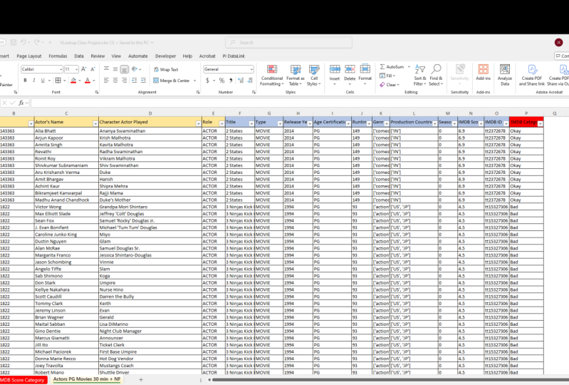I also have those within this project resource workbook. Alright, so I have a workbook with three tabs. And these three tabs are all related to Netflix movie data. Okay? Our first one here is a list of Netflix actors who played roles in all Netflix movies and shows. It's just a complete list of all, of all actors. Now, our next tab is called Netflix movies. And this tab in particular is showing only the Netflix movies that are rated PG and have a 30-minute or more runtime. And then our last tab. This is a custom category grouping of IMDB scores. So what IMDB scores are just basically movie ratings that viewers give two movies, okay? So we have these three spreadsheets and they're all related to some extent. So what our mission is here, we want to create a brand new table. In this table, what we wanna do, we want to show all of the actors who had roles in these Netflix movies shown here in this list, which again is a list of PG rated movies that are at least 30 minutes or more. So for example, I'm going to filter to one. What's one movie will filter to three ninjas kicked back. In my new table. I want to list of all of the actors who were in that movie. Okay? Alright, so let's jump in and I'm going to demonstrate exactly how we're gonna do this project. So step one here, I am going to duplicate the Netflix actors spreadsheet. Because the goal is to have a whole list of actors who were in these particular movies, right? So we need to start here. This is where this is going to be our starting point and we're going to build off of this. So what I'm gonna do is just right-click on this tab. And I'm going to click Move or Copy. And I'm going to move to the end and click Create a copy. Now that I've created a copy, I'm just going to hide the old one because I don't I don't need it anymore and I don't want to get confused. So I'm going to right-click on it and hide. 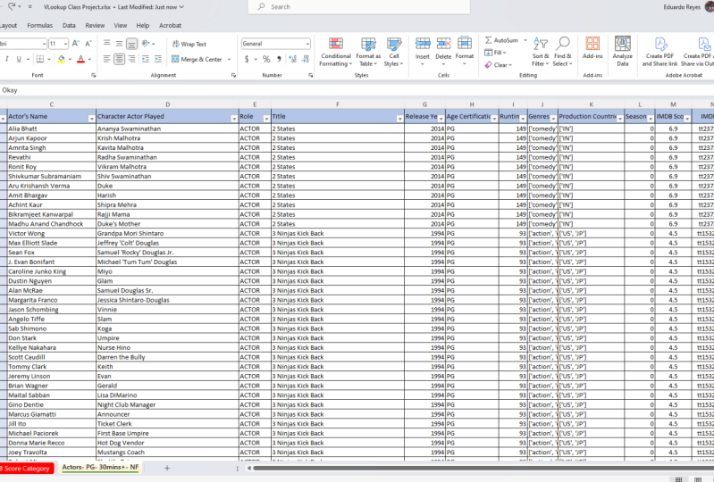Okay, next thing I'm gonna do is rename this tab just so it's clear to what it is going to be. So I'm just going to name it actors, PG, 30 minutes plus movies. And F standing for Netflix. And you can name yours whatever you like. Okay, so now we have our new tab and I'm going to just change the colors because I like to distinguish my new my new tables or data from my other data. Alright, so I'm just going to make it green. Alright, so the next step here, I want to bring in the Netflix movies information. So all of this information over to my new table. Now, in order for me to do that, I need to find a lookup value that is unique and exist in both tables. So I'm going to look at this particular table. I have a person ID and I have a movie show ID, and then I have actor information. Now when I go over to my Netflix movies table and see what I have, I have movie show ID, and it looks like I have movie information and also an IMDB ID. So what do you think we're going to use for our lookup? If you guessed the movie show ID are correct because that is the ID for the movie, right? If I just click on one of these IDs, it is showing all of the actors and actresses that were played roles in this particular movie. But we don't know what movie that is. We only have the ID. So what do we want to bring in all the information for that movie? We're gonna do it by using this ID right here. Because it exists in both tables. Alright, Now before we perform a V lookup, one thing I want to look at here is the information I want to bring in, okay, So I want to bring in all of this movie information. But we have one problem. I know a VLookup is always going to look to the right of the starting column, right? So when we're referencing the table array, I'm only going to be able to bring in this information. Well, we have the title over here. So that doesn't work. I need the title to be to the right. So what I'm gonna do is just right-click the column a where the title is, and I'm going to cut it. I'm gonna go over to column C, highlighted, and right-click and insert. So now I'm good, right now when I, when I reference this starting column for my table array, I can highlight all of this data and I'll be able to bring in with my VLookup so we're in good shape there. So the next thing I wanna do is look at these IDs that I will be using to link these two spreadsheets together. I want to look at the information in here and see if it's if it's a number ID or if it's a text ID. So we can see that these are texts IDs. Okay? So if these were spreadsheets that I knew the texts were 100% the same, I wouldn't have to do anything here. But because in this example in particular, I didn't create these spreadsheets. I'm going to trim both of these columns just to ensure that they are exactly the same. Okay? So for example, you can even see right here in this particular cell that this movie ID has a space over here, right? Where the other ones don't. Okay? So we're gonna use our trim formula to take care of that. So I'm going to start in my new table first and just insert a temporary column. And I'm just going to type equals trim. And I'm going to click in cell B2. Close it. All right, Now I'm gonna double DoubleClick to drag that down. Make sure everything worked it did. I'm going to copy. And then I'm gonna come over here to B2 and paste as values. Okay, and that, that trend, that column B. So I'm going to delete my temporary column. And I'm gonna do the exact same thing for my Netflix movie spreadsheet. Alright, so I'm going to insert a temporary column equals trim. I click in cell a five, close the parentheses from a formula, double-click, drag it down, copy it, come over here to a five, click, paste these values. Perfect. Now we can delete that temporary call. Awesome. Okay, so now we're in a good place. We're now ready to perform our v lookup. So what I'm gonna do here is highlight all of these headers. I'm going to copy them. And I'm not going to highlight the movie show ID1 because I don't need that, right, That's, we're going to use that for our lookups. I'm just going to highlight the ones that contain the date I want to bring in. And I'm gonna go over here after I copy it, go to our new table. And we're going to click on cell F1 and paste it. Now the next thing I'm gonna do is make sure I have filters on all of my headers. So I'm going to click in here, highlight all my filters. I'm gonna go to my sort and filter button. And I'm going to click on Filter and then go back in there and click it again. So now I have filters applied. Next step, I'm going to highlight these columns and just make sure and there in general format so my formulas will properly work. 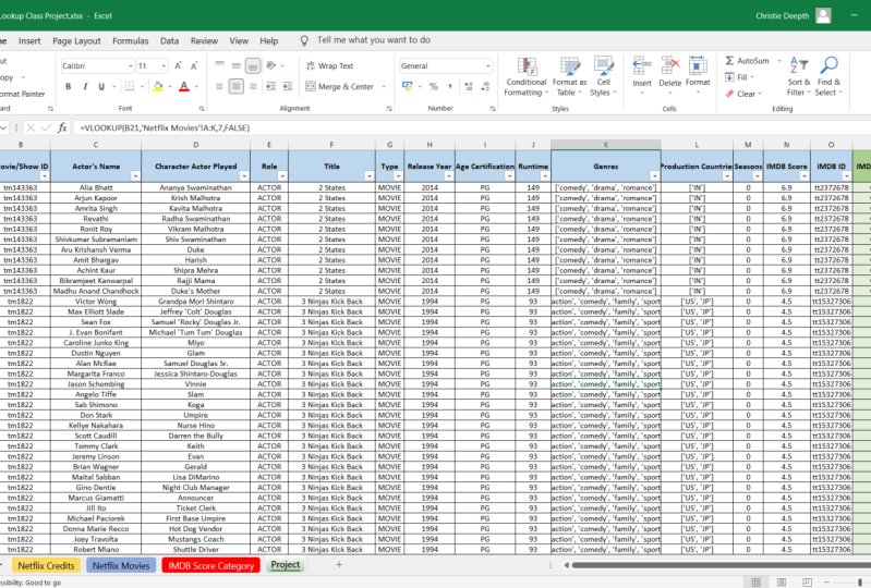Alright, so my next step is writing my VLookup. I'm going to start right here in cell F2. And I'm going to type equals V L. And I press tab. Okay, what do I want to look up? Well, I want to look up the movie show ID, so I'm going to click in there. Press comma. Alright, Where's the table array that I want to look for it in? Well, I'm gonna go over to my Netflix movies tab. And we want our, we want to look right here, right in column a. Okay, great. If we do find a match, what do we want to bring over? Well, we want to bring over the title so I can stop here. And then we'd be good. But we're going to use our shortcut that allows us to copy and paste the VLookup to all of our columns. So instead of stopping here, I'm going to highlight everything all the way to call them K. Okay? And if you look closely, we can count the columns. Titles in number two, type is in 34 and then so forth, all the way to 11. Now because we copied these headers in the same order, we see them here. It's going to save us some time when we copy and paste our v lookup. So let's do it. I'm going to highlight all columns up to 11. I'm going to stop there. I'm going to press comma. And now I know I'm bringing in the title. That's the first. A column of data I want to bring in. So that's the second column. I'll press two comma. We want exact match. Close it. Okay, now it says NA, but don't worry about that. We'll address that in a minute. So now that I have my formula here, I'm going to copy that formula. So I'm going to click up here at the top of the formula, bark, highlight it, and press Control C. And then I'm going to click once and sell G two and press control V. And then we're gonna go over to the next cell. I can press the Tab key, press control V, tan, Control V, tab control B, control V, and so forth. Alright, so now the next thing I need to do here, because remember we copied the exact formula where it shows a two. So all of these are showing the column index of two, which is for the title. So all we need to do now is just change that to, to the next column over. So I'm going to put a three here. Press tab. And the next one I'm going to put a four. Next one, I'll put a five. Next one we'll put a six. And you get the drill here, 78, press Tab nine, press Tab 1010, press Tab and 11, or 11, and then go to your end of your formula and press Enter. Okay, So now that we've done that little shortcut and we have our VLookups ready. I'm going to highlight all of these VLookup formulas right in this, in this row two. And I'm going to go to the very end double-click. And now I, VLookups are going down. We have, they went down the entire spreadsheet. In this example, I don't want to see the formulas anymore, right? I just want static information. So while it's still highlighted, I'm going to immediately right-click and copy, and then right-click and paste as values. I'm going to choose that clipboard 123. Ok. Now you see all these NAs and you might be thinking, okay, why do we have an ace? Well, remember, we started with the entire list of actors. It didn't matter if the movie was under 30 minutes or if it was not rated PG, it was just all of the actors who are Netflix shows and movies by the way. So that is why we're seeing NA's. Now we know we only want to keep the ones that are associated with these Netflix movies, the ones that are PG and 30 minutes plus. So all we need to do now is get rid of R n rows. And the way to do it, very simple. I'm going to pick one of these columns. So I'll pick the title column. And I'm going to sort a to Z and or z day. It doesn't really matter. We just want to make sure it's sorted so all the NAs are grouped. And now we're gonna go back in there. And we're going to uncheck Select All. And then we're going to scroll down to the very bottom where it shows the NAs and we're going to select it. And now we're gonna delete those rows. So I'm just going to select this first row at the very top. And I just clicked right in there. And I'm going to press Control Shift down. And I'm going to right-click and click Delete. And then I'm gonna go back into my title filter and select all. And we're done. Perfect. So now we only have a list of the actors who were in these specific movies that again, are rated PG and have a runtime of at least 30 minutes or more. Alright, so what I'm gonna do here, just to make it look clean, I'm going to select all of this new data that I brought in. And I'm going to apply some borders to it. And maybe I'll a left line it. Okay, So what we can do now is we can hide our Netflix movies tab. We don't need that anymore right? Now. We're only playing with these are new table and this category mapping table. So what we wanna do is take a look and see, okay, how do we link these two together? Because we're going to have to perform a newbie lookup. Well, we have an IMDB ID and we also have a score. Okay, that's good. Let's look over here. And what do we have? We have an IMDB score, and that's it. That's all we need, right? We're trying to map the scores to a category. So all we need to do is look up the score here. From here. Alright, perfect. So let's make a new column right here. And I'm just going to simply highlight the header and right-click copy. Go over to our new table. I'm going to right-click paste, make that a little bigger. And I'm going to make sure it's in general format. Now, the next thing I need to do before I do my VLookup is take a look at my lookup values. And again ask ourselves, is, are these numbers or are they text? Well, these ones are interesting. We can see that this one is text actually. It says 1.8 and it's, it's in text format. Now, if you are not sure, it's always good practice just to convert your numbers to actual numbers or your texts, actual text. So I'm going to highlight my scores. And I'm gonna go to my Data tab, Text to Columns. And we're going to click Next, Next and Finish. All right, Perfect. Now let's do the same thing for our mapping spreadsheet. So I'm going to highlight those scores. And I'm gonna go to Text to Columns. Go next, next, finish. Perfect. So now I know those are the exact same format. So now I'm ready for my last step here. I'm going to click in cell P2 equals VLookup. What am I looking at? I'm looking at the IMDB score. So I'm going to select n2 and then comma, press comma. Okay, where, where am I? Where do I want to look it up? I want to look it up here. And then I want to bring in the IMDB category, which is in the second column over. So I'll highlight that. Press comma two, comma, exact match, close my parentheses and perfect. So I'm going to double-click down there. And I'm gonna make sure I apply a filter to that header. And we're good. We can see that we have all of our categories listed. Alright, last thing I'm gonna do is just by my personal preference, I'm going to put some borders on it and maybe I'll change the color, whatever whenever I want to do. And we are all set. All right, so good luck with your project. Again, if you have run into any issues, feel free to re-watch this project video and definitely utilize your step-by-step instructions. And I really look forward to seeing your finished projects.