Excel Data Analysis with Microsoft Excel

1. Introduction: Hello everyone, welcome to Excel data analysis with Microsoft Excel. This is Ali had done and I'm going to be your instructor during this class. As a prerequisite for this course, you just need simple, basic Microsoft Excel skills. For example, how to open a file, how to save, how to enter data, differentiate between the column and the row, just the broad skills and stuff because all specific tools or commands are learned or are explained during the course. For example, how to use the split formulas, how to use the sum, or how to sort the data that you have, or how to use conditional formatting. So don't worry concerning this topic. At the end of this course, what to expect. You will be able to gather and describe data and analyze them. Also, you will know how to use advanced statistical tools and make decisions on operations, risk management, and finance. Concerning this course, you will see that each project or each concept is accompanied by supplemented exercise or assignment in order to make stuff more reliable and more read. Because data analysis is highly related with their life problems that we have or the main workflow operations. So it will be very enjoyable and interesting. The fourth objective of this course is that you will enhance your analytical and logical reasoning. Also learn about project life cycles. For example, the risk management, the criteria, the fraction of the criteria. Everything will be more clear during the class. And also you'll learn how to build an analytics framework and use analytics tools to draw Business Insights, define it to objectives are mainly explained and achieved in the final concept, the problem-solving. As an outline, you will learn how to use the payroll. The payroll, for example, let's say you are a company man and trying to pay your employees and keep track of their overtime. So that's what we will be doing inside this project. Also the grade book. We will setup a great book and we will be doing a computing and percentages. We will be finding who's in the top of our glass and who's not. And also the third outline made outline as the factor Decision Tree program. So we will try to decide what carrier would be best based on what we prefer, what the pay is and other benefits of your job. So we have different criterias and different fraction for each criteria to do so, a spreadsheet will help us determine how to make a decision. Also, another application is that we will create a sales database. So I will give a bunch of data and who will sort that. We will determine what are the, who are the best salesperson, what is, has commissioned and make some charts, exception of charts, that we will talk about. A very interesting topic, the card inventory, where we will create what's called a database actions. We're going to have a large number of data again, and we can show you how to concatenate, to feed into how to split them, how to make reports with this, this is very essential as your are in a place or any stock manager because you, you will learn in this section how to create the item ID. The final section will be as reserved for different problem solving that we are going to solve. So the first four projects are more tutorials to show you how something is done. And then I'm going to give you a challenging assignment at the end, where I give you half of solution and then you use your creativity in what you've learned in the previous explanations to see you if you can solve the problem. And so both we have a tutorial section as well as the practice section where you can put things into service at the end in case you need to any question, any elaboration or do you have any suggestion for future courses? Please do not hesitate to contact me through my e-mail ID Hampden D21 12 at hotmail.com or through my phone number. It is a Lebanon's. So in case you prefer to talk through WhatsApp Telegram, I'm open to all options. And in case these applications were not available or did not fit, I do not hesitate to contact me through my LinkedIn. I wish you the best of luck, and I wish you enjoyed this course. Please. Don't forget at the end to keep me, to keep your feedback for any future suggestions or recommendations. Thank you and enjoy your discourse to the maximum. 2. Payroll: Hello everyone. Now we'll start with the payroll. The payroll can be used by any HR or any person that works, any company that will manage the payment and the overtime of a whole group, it can be used by a team leader. For example, if I have a company acts that has four groups that are working, and in each group We have 20. We have a group manager or a group leader that he has to put all this data and something called the payroll. Okay, that's perfect. We will use Excel for this concern. Let's start with creating the lastName. Then the firstname. Firstname, then the hourly wage. Let's greet him here. Hours worked and put one, John. Okay. That's perfect. Move on to the hours worked. Now, the payment that it should be put in order to make it fit, I have to press it like this double-click or I can run it as much. I won't. The same as here. Okay, Let's start with mon, dark. One. I will work on a group of 50 only to just save time. Mon Jack part bats. Central. Carlos. I'm done here now we'll move to Malawi. Since the hourly wage depends upon your position, let's say 15.912.26.49.11. And here, then pointing to the hours work in January 1, let's set a random or not random, a fixed hours related to each employee. So the fourth, they should work 40 hours per week. We have some overtime, 4430 to 4041. And here, 46, here. Now we'll start with the PE. Let's increase a little bit the pay and you create a formula. So we'll start by pressing equal. Equal what? Each hour times no, excuse me. Each but each employee it's hourly wage times. Times what times? The hours that he worked. Excuse me. I did a mistake, not the D7, D6. Okay. We have that. Jackman has 699.6. Let's create it as a currency. So we select the whole fit or the whole cell. And create here as a currency. The same for the hourly wage. Okay, That's perfect. As 699, I can do the same by pressing equal times 32 and drawn it. However, we have something more easy. I can copy it, I can copy and press here as a biscuits. And this can be done also in another way, in a nice easier way. Let's remove those. Okay, I can take its corner, it's lower coordinate and run it till it fit every section I want. Now let's move on to the section where I want to implement some functions. For example, if I want to create the maximum, if I wanted to create the minimum, if I want to create the average, also the total that I won't. It can be done for each one. How I do such functions in a very easy way. I can press equal. We have inside Excel a very large library of functions that we can use easily. So we press equal max, not equal max, excuse me, equal max here. And now I press he needs number one, number two, etc. All the numbers that I want to compare, I want to compare from this number, then this number. So he pressed he tells me that 15.9 is the maximum hourly wage that John Mack Jack bond gets. The same for the minimum. Minimum. Excuse me, equals min minimum, it returns the smallest number in a set values, ignore logical values at texts. So the minimum is repress the parenthesis and we select the area for sure. Close the parenthesis at the end. We have that 6.4 is the minimum hourly wage took by Carlos syndrome. The average is the same. So if I want to press average and the average we have different and a large list of averages. However, I want the simple average formula. I can have to choose the set of numbers. And, and the parenthesis is 10.7 to the company in the payroll PDZ, on average, $10.72 as an hourly wage. The total, it's easy. The same, one, total equal total of this one. I know this is wrong because many people believe that just creating, putting the function that I want, I will find it in Excel and this is not the case. The total is not presented in this Excel, so I can not create doted. If you can see that before I didn't reached any function. There is no, nothing called total. So it is easy. I have to press plus this plus this plus this one. No, not this one. Plus this one, plus this one. It can be done in an easier way. I can do it another time we found a typo in your formula. Okay? Yes, it's correct. As a company in this group, they pay $53.61 each hour for the employees. This is not a very big number. So we can continue it the same here. We get that the maximum is 56 hours, the same as here. We got that the minimum is 32 hours by parliament that has an average of excuse me. I moved it. As an average. We get 40.6 hours each employee work and the total is 200, three hours. There is something wrong here. I believe that you saw it easily because we inserted a copy from this section. And this section is in currency. So we have to change what we have here to gender numbers. So we go up there and we change accounting to general number that I want. I can have, I can have a berry list of numbers such as generals, such as a number such as a currency and accounting as short date, long date time percentage, fraction, scientific fraction, or even tax. We have even more number formats that we can find that in this section. Let's not our main concern. Let's move on to the maximum, minimum average total of the pain. So I can easily Move on panel excuse me. I can easily move on these ones here and get that the maximum is 609 earned by Jackman. This is can be understood and the minimum, the average, and even the total. However, also I have to change the currency here, $2 to make it as an accounting. And in case you face something like that, that the numbers are not faced. Don't panic. This is simple. You have to enlarge your cell in order to fit the whole numbers. And this is as an assignment, One concerning the payroll. This is not complex, not hard, and it is easy. Now, let's make it a little bit more spicy and insert the overtime. How we insert the overtime. If I want to go to E and I want to insert a section in E. So this section here will be pushed to the right. I go to the, to the block E and press right-click, Insert, and we got a new section or a new block called E. I have to say that it is the overtime and that the overtime is in 11, John. Okay. Perfect. What is the overtime? Overtime is every hour exceeding the minimum hours worked by an employee. So the minimum hours worked are 40. So I can create a formula for that equals to the hours worked minus 40 and press it. As for Jackman, he worked only four hours, which are the 40 the required ones, and the four which are the essential ones. If I want to move it along the whole section, I can see that since Holloway good. Six even got one hour, Carlos got 0, but Paul got minus 8. This is not the case because sometimes in work areas or in work sections and companies, there is no lower over time. It depends on the policy of the company. However, if you worked less, it may because of excuses, of reasons you are sick, you travel jar taking your annual vacations. This is not the case. So how do I have to change that in case it was negative, I have to make it as a 0. I have to press the value 0. This is not the negative over time. This is not the case in our working place. So what we do is we create something called the F formula. And this is mainly used in the payroll for the overtime. So instead of pressing D6 minus 40, I have to clear my section. Let's right-click and clear content. Now we go and press equal. If, if what checks the function, checks whether a condition is not and returns one value if true and another value if false. So this is what we are searching for. If we have the logical test, what is the logical test? If the hours worked are greater than 14? What we put it, what we returns, we return is now the value if true, the value of true is the 44 minus, excuse me, the 44 minus 40. And then if the value of false just return 0. This is simply, as you can see, if the works, the hours worked are greater than 40. It will return a value. This is a programming, a Boolean value, true or false. So it will returns a value true or false. If it is true, it will apply the function, the D6 minus 40. If it's wrong, it's false. It returns just 0. So let's enter it. We will have four and nothing will change unless the negative value where that part work 32 hours. Here, instead of getting minus 8, we got just a 0. This is very essential for you to work on and understood and understand correctly. Now, by this, we finished the overtime, however, in January. And as a manager or an HR or a company man, you give a bonus for each employee that works over time. For example, if you worked on over time through the mid night, you will get a bonus. So in general, I searched on the internet and I saw that the average is 0.5 plus the hourly wage. So I have to create a section here, and it will be the total paid. The total pay will be the following. The total pay will be equals to the January pain that we have. Plus plus what? Plus the hours worked times? Times what? Times 0.5 of what? Of the hourly wage? By this, we got that a Jackman take 731.4731. Let's run it to everyone. We can see that bar and bat and Carlos and drill got the same pay and the total pay with and without the overtime points. So let's run it here. Excuse me, cuz me, no, no. I made a mistake. Not a big problem. And let's run it here. Don't panic. This is simple. You have launched a little bit, enlarged more. We have that the total is 2245.87. Now, what if we want to work on a greater number on, in greater workflow? Let's assume that we have not just one January, we have to work on age annuity, 50 ingenuity, and 22 January, even 29 January. What do we do? Let's press that. We insert section here, another section here, another section here. Even one more section, and an additional section. Excuse me. So to work on this one, I have to press the hours worked in order to not put ingenuity 15 January, we can create a simple formula equals this one was seven days I want As a week. So I got eight annuity. Let's move on here. It will get me to excuse me here, 15 January. And now 22290 annuity. This one, I can easily delete it. Okay, This is simple. Now let's insert how much time hours worked in each in each week. So let's just assume 4542. He took some breaks, 34 and here, 40 excuse me, the 40. Now we get 42. Forty five forty six, forty one here we've got 32314049 here rather than down works forty five forty six forty two. Forty seven. Okay. And since we worked forty three twenty nine, thirty eight, and thirty 23. Okay. Now we can do the same that we did earlier, but for a larger scale. So here instead of inserting each section alone, because even the overtime has five sections, so I want four sections. Okay. Perfect. I I select the four selections and press insert or excuse me, know, I want to shift the sens, right? Excuse me. Insert shifts. I was right. I want to select everything, sorry. And here, insert very easily, I can recreate the same formula plus seven and along the whole month, 2900 annuity. Now, I know it's easy that we can recreate the overtime for every section. However, this is not practical because you are using Excel in order to compute, to run stuff that takes time with you, boring stuff with you, and just simple way. So what we will do is we will press as equal to the hourly wage times what times the age annuity. And let's excuse me. No, no, no, no, not this one equals the overtime equals if the logical test, if it January greater than 40, now, we press as d minus 40 and the same will be 0. I already taught you this formula. Let's run it along the whole employees. If I want to compute it, I will get the same here and here. That's perfect. I can also extend the stuff. Okay? Let's extend them from here till here. Even though over time, it can be easily done. So I can get the overtime. Why this overtime is 49? No, no, no, no. The maximum is 49. Okay. Perfect. This is for the overtime. Let's move on to the pale. Okay. Let's create a section for the pay. And here press one, January. Okay? Let's move tidbit right? And put us 1, 2, 3, 4, insert, we get this one equal one January plus 7. The same formula. I'm just reapplying them as that. Here we have something new that you will learn in this section. Let's tell you what will be the pay for the first object. Annuity is the 14.9 times the hours worked. I would apply the same as I will reuse this one and get it till here. I will have that. Suddenly I am facing one hundred nine hundred eighty, around 2000 dollars each week. This is not logical because if you want to see that 45, it's just one extra hour worked with Jack bat. So this is not logical. What is the main problem? If I want to press here double-click, I can see that the C6 and the D6 are colored by blue and red. The same will be here. Let's check what that Excel understood when I shifted or I took part of the 1st January and I run it along the right. So he understood that he moved even this one to the right. So he multiplied the hours worked in the first of January and the eighth of January. This is not the case that I want. So what we will do now, we have something called the absolute referring, referring Excel here as a default, he understood that we are using the relative referencing. So if you move one to the right, he takes everything one to the right. This is not our case. I am willing to multiply the hourly wage for each employee by the hours worked in each week. So I have to clear my content here very easily. Radically clear contents, and I have to change something inside my formula. How to tell Excel that I'm modeling tools, absolute drafting. I want to tell him, I want him to understand that the hourly wage will be multiplied by each hour hours worked in each. Week. So simply, I have to press the dollar sign before the section that I want to fix it or to make it as a just fixed one. It will not move to the right as the relative referring. And now let's check it. Let's check. If I want to run it, I will have nothing changed. And now I can run it easily. And here I can see that if I double-click he, uh, he multiplied the hourly wage by the 8th of January, the same here. This is very smart of Excel and some people do not know it even if they are expert in Excel. So by this, we created everything. Everything was simple. Let's move along this one and let's continue. Okay, I'm going to minimize a little bit smile vision. You can minimize it here by view and zoom to selection, also, unzoom selection, zoom to as 50 percent, zoom as 100%. That this, you can use whatever you feel it as easy for you. I will use the one, the one in here, 85 percent. And this is very practical for me. And I have take the total pay, do the same for the total pay concerning that I did for the PE that's as first of January. And here we create a formula. No, excuse me. Here we create a formula equals 2, this 1 plus 7. Let's move it a little bit along this one. Okay. One more one more week. No. Not fired for query. I'm just concerned with the January. Okay. Here, I want to create a new formula. What is the formula of the total pay? The formula of the total pay is equal to the pay that he took. Ok. Sweet. At the pay that he took an age annuity plus the overtime hours times 0.5 times the hourly wage. This is the same if you want to proceed here, it is very logical. If I want to fit it to the right, it will be the same because he is taking the As here. He's taking excuse me. He's taking the hour worked as a wrong. So we also have to use the absolute traveling to do so. So I'll go back there and press at the C6 as a reference one. And here I can move on everything. Nothing will change. Here. Some stuff we'll change. This is very logical, and let's press the ingenuity. We can see that it ran the P6 the first day, 15 January 1, times the K6. This is correct. Times 0.5 times the Howard League, which this is the same for 22 of January, he took the hourly wage as a fixed one. I can use the stuff and run it here. Let's fix them a little bit. I highly advise you to work on colors. So let's start by the lastname, firstname, and the hourly wage. As a first section, we go to Home and we have the styles section. Let's make them as a neutral. Here's the hours worked. It will be, let's say bad and read. The overtime is something positive. So let's put it as a calculation. Just the orange section. The pay one checks and the conference at that. Okay. It's okay. And the total pay it will be for showed in green because it is good. So this is everything that we have concerning the payroll. And I wish that you've benefited a lot from this section in case you need any extra stuff concerning the payroll. If we want me to set it as greater level, higher level, please do not hesitate to contact me. Thank you so much for listening. And let's move on to another section. It's very important sections concerning the grades. 3. Gradebook: Now arriving to the grade book section. In this section you will learn how to make comparisons between a series of components depending on another series of criteria. So I will assume that we have 10 employees. Let's just fill another more five. Additional five. Okay. Say brac, Sandra, let's say also selling crack. Berlin, seat set up. Okay. Even we have these R3 shape. I need two more. So Raquel, Sebastian, self. Peter. Okay, perfect. It's better, not be bitter. Okay, perfect. Let's make it capital. That's perfect. I am running for tests. Okay, perfect. So the first task will be the safety test. The second one will be the company. Let's increase a little bit. Let's zoom. Okay, So view, that's running Zoom to the 100%. Okay, even you can do it as a greater so safety test. We have the company philosophy asked. The second one will be the financial skills test. The fourth one will be the drug test. So in order to be more accurate and give correct answers, Let's give each dust the points possible, the maximum points possible to do so. So let's maximize those. And these four, we select them, we go to home, then go to this one, the orientation, it rotate your tax diagonally or vertically. This is a great way to label narrow columns, so I will rotate it as angle clockwise. This is perfect. Let's run them a little bit. Okay. This is the one and this is okay. The safety test. Let's give it as a tan, the company philosophy, let's give it as a 30. And the financial skills that give it a 60. The drug test it is just over one because it is either you passed, you get to one. Either you failed, you get 0. So there's no chances. Let's start giving points to each one over the safety task than 9898357689 and 10 over 30, Let's 2829. Okay. Good. 2009, 25221517. This is, let's say 22 here. Let's put it down. Here. It 12151725, the financial skills test. Let's give four hundred fifty four fifty seven. The financial skills, Let's give him a 28 here, a 35 here, a 39 also here. And let's give him a 59 here. Fifty two, fifty three. Forty four. Forty three, forty two. And here as a 60. Okay. Perfect. That drug test all passed on. But this $0.01 Alawi did not pass that. Are okay. And here Let's hear what. Okay, perfect. Now we have the four tests. Let's start creating a percentages of them. So I will copy those, copy and here I will press a based. I will have the same tests here. Let's adjust the shapes. Okay, That's perfect. Ok. So what we will do it now as we create. An equal, this one divided by this one, and print it as a percentage. We'll get 100%. Let's continue and see where we did a mistake. We continue. We see that it is 90, 167. This is correct. 9 over 10. However, here nine over ten is not a 100%, and here eight over nine, this is not the case, so we have something wrong. Let's suppress on the wrong stuff. That the first one, the nine it is over the ten. This is what we called previously the relative referencing. So what we have to do is to create an absolute referencing simply by pressing after the d, the dollar sign. And here, let's reorder them. We got the correct answers of all of them. Let's press the six. Is six over 10, the 100 as the 10 over 10. So it is perfect. We will do, excuse me, we will do the same for the company philosophy. So it is equal to 29 divided by this one, however, depressing a dollar sign to make it as an absolute referencing. Okay, for sure you can create it as a percentage here. Let's move on. Let's press it there. So here we can see that it is 54 over 60 here, 35 over 60. This is correct for all stuff, we can see that the drug does either 100% or 0%. So there's no big deal concerning this topic. Now, let's give it some spices, some funny or amusing stuff. We go here to the safety test, and let's press conditional formatting. It is in the styles and the Home section. Conditional formatting, we go to the icon sets and here we have some stuff like the shapes of the four traffic lights. You can choose a set of icons to represent the values and the selected cells. We can see that the tan got a green light, even the nine to get green light, the average one's good. Got eight. The red ones are 5 and 6, nearly ordinarily above the average on the, the one who failed took a tan. You have to condition each one at at each because each one has a set of different stuff, please. This one is not conditioned. Clear roots. Okay, perfect. This is the selected ones. We will do the same here. I concepts, okay, will do also this one. And the drug test. However, I am doing such stuff. Just to get an answer why I'm doing these tests, because I want to fire an employee to see which one is the best employee, etc. Let's continue conditioning. Let's start here by Select All. And let's see which one got a less than 50 percent in any of these tests. So I will go to conditional formatting, but we will do highlight cell rules and repress less than, less than what? Less than 50 percent. That's perfect. We can light it light red, yellow fill with dark. I will keep it as standard one, light red fill with dark red text. We can see that this one batch body that failed in the financial skins dust ham than Ali failed and the safety test hello isn't failed and the drug task, even Brock sand drains and in Rock failed in the company philosophy does. So. What we will do now we will create a new section called fire employee. Employee. And let's oriented. That's nice. Okay, it is oriented and we will create a condition. The condition here is the old condition or condition. I will tell Excel to check if there is any of them. Any of the four dusts did not meet the condition that I will insert. So I will press equal, or it will checks whether any of the arguments are true and returns true or false. A Boolean value, it will returns false only if all arguments are false. So here we press, or this one is less than 0.5 or 50. 4.5. How big did he will understand that? The second one, if this one is less than 0.5 posts. So if the financial skills as less than 0.5 comma F, This one is less than 0.5. Ok, we can see that it is false. Do I have to file this employee false because all of the safety the older tests where Matt above the average that I set as 50, each company or each HR can set his own criteria as columns corresponding to this task. So it is not an ideal case that I am using. So Let's continue and run all the stuff. We can see that part of it, but I have to fire him. Even Hampden ALI, Allah, we send Brock, Sandra, and croc selling. These employees did not meet the correct ones in order to make it easier. So let's select them Conditional Formatting, Highlight. We can, if it is true or it is wrong. So let's see this one. I didn't appear. So let's see this stuff by not appear. Okay, no big deal. I can format it as highlight. Which one if it is equal to 2, highlighted in red. Okay, perfect, That's the end of this section. However, this is the main idea when it comes to firing the employee or not. How about checking? What is the maximum, the minimum and the average is also simple. We learned them in the previous section. So the average here, I press equal max of this data. Here the Min of these data. And here I press the average, the normal average also of this data. Let's press them. Remove this and here. Check it. There. I got that a 90 percent. I can press here the same and copy here, paste it. We can see that it gave me through numbers. I can go to the home clipboard font alignment number to the number section and press the person style. You can also press it by Control, Control Shift and the percentage is also clicks. You look more advanced in Excel. By this, we finished the maximum Min and average. However, as we can see that five employees that not meet the four tests, the required criteria out of the four tasks. So in general, HR's prefer to have charts concerning this topic so you do not adjust, choose only one criteria and take your decision over it. So we go to Insert. Here we have the Insert Column Chart, 2D column, the short title. Let's call it as the safety test. The safety. That's the x axis. The x axis will be these employees. Okay? Okay, Excuse me. Select data I wanted from here. Let's go to the employees from here till here. Okay, That's good. Select the data. The series that acts at the y-axis, excuse me, the y axis should not be this one. The series name. The y axis should be the safety test. This one's the series value. Those ones. Okay. And the x-axis would be these employees are Press Okay. We got it as, as following here. Press it here like this. Let's create another chart. Insert. We go to the charts, I will choose the first one, the 2D column. Know what result. I will select data. The y-axis will be without a name, the series value will be the following. Here. Perfect. And the x axis will be the same people here. And I will call it as here. Let's copy it because I deleted in the wrong way. So I will call it as excuse me. Let's track the company philosophy, dust. The company philosophy. That's okay. You can see that we inserted different stuff. Okay, perfect. Now let's continue with the third chart. Insert chart. I'm setting this range. Excuse me, Select Data. The data the legend series will be the financial skills one. No, this is not the series name. This is the series value. The series name will be the financial skills dust. The horizontal data will be from 1 to circle. Let's run it. I got it as the financial skills test. So by this, we created three charts. One, concerning the company philosophy tests and the safety test because I'm not firing people because they didn't know the company philosophy test didn't pass it. However, I may fire them if they failed the safety test or the financial skills tasks. However, the company philosophy tests, I can do just like a comparison between the safety test and the company philosophy test. And if a person that passed or not passed the company philosophy tasks, however, he had a very high grades and the safety test. I just can't keep up with him and compute some trainings or increased his skills concerning the company philosophy test. For sure you can make some styles here, neutral one. Here, the percentage, what are the good ones here? Let's make it as a calculation. That's very nice. By the way, the max and Min, I can put them as Chuck cells. And here I can create it as a heading. So hearing increase it a little bit. This is ready. Here. I can press it as an accent to increase it. That's perfect. Let's go to File Print. And we can do different stuff. I can make it as a no scaling. I can fit sheet on one page. I can print the entire workbook, the selection. I can change the copies, even the pages. I can press them, even the paper orientation, it can be done as a print, as a landscape for sure, I highly advise you to always use the landscape orientation when it comes to the printing. Now we go to the SLB MUX. This first concerning it is advanced a little bit less skip it, and then Orban margins can be changed depending on, uh, your selection. You can choose it as a normal one. You can choose that as white, even as an arrow. The top, the left, the Hadar at each section can be identified in the Custom Margins. One, you can define the stuff and even you can use some artificial intelligence, such as the feet of a treat on one page, fit all columns on one page and fit all rows. By this, we finished the grade book section and we will move to another interesting topic. 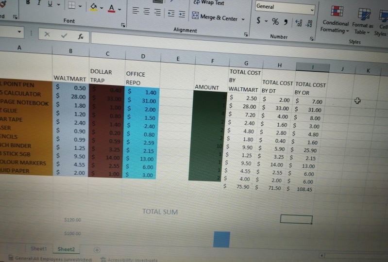4. Decision Maker: Now arriving to the decision maker part. And this part, we will work on creating a scenario in which where we are supposed to pick a job and you're going to weigh different factors based on our opinion or your opinion. So you can change from the data or from the concept or a list of jobs that you are concerned. So beta amount of jobs that are out there in the job market, how much you enjoy it, how reliable the job is to you at various factors. And then based on European Union, Excel will give an answer on what carrier you should choose. So let's talk about the career decisions. Perfect. Let's minimize it a little bit. Okay. That's good. So let's start by listing the jobs. So the job we have first, the manager, we have the doctor. You can change the jobs depending on your choice. So I'm choosing the most common five jobs, the teacher and the driver. Here we will put our criteria. Our first two criteria, criteria will be the pay. We have the job market. We have also the enjoyment during the job. Are you enjoying the job or no, even newer talk about your tongue. It takes a part of it and the schooling. So let's start by adjusting a little bit. Okay, no, I'm going to put them on my editing. Okay, perfect. And now we'll just give the random values depending on your choice. So if you are a student, you didn't reach the university. This is very important for you to check if you really enjoy the job or the major that you are getting involved and so forth to. The talent requires 42342, the schooling, it requires 51335 for sure. This is not correct and let's put it like this. Okay. By this, we put that talent. We will put the criteria upon which we will choose our perfect job. So let's create something called the total and press equals sum. I previously told you that there is no variable or function inside Excel that is concerned and the total. So if you press total, it will shows nothing. So I didn't give you, gave you the valuable that you can use. However, this is the sum. So I wanted you to the basic one, the plus, and even somewhat. So. In the coming section or assignment, you will see that there was a, there have been a cause behind this thing. Now we have the total 12. I can run it over all. I can see that the teacher is the best job. However, if we want to be realistic, we can see that each criteria does not take the same proportion or the same importance factor. So I will create an important factor. Let's insert after each criteria an important factor, depending on it so that the pay I will give it as A3. The job market will take truly a five because if there is no job market, there is no, there is nothing, there is no job. So it takes a big factor. The enjoyment is sport, just to pursue. And at the time that requires a three and schooling is not the important factor. So schooling, I will give it a one. Now let's create a function that will multiply each grade and depending on each criteria with the proportion or the importance factor of this criteria. So I will create it as equal to C4 times one. And we already talked about it and we already explained that a lot. We need an absolute referring concerning this thing. So we insert the dollar sign here. I can run it. I can copy, paste it here. It will be the same. Okay? For everything. Okay. That's perfect. If you can see that the total is not correct because I want to calculate just the values that are concerned with the importance factor. That's why I didn't told you about the sum because I wanted you to understand how we do the basic math using excited because in some areas or in some spots you cannot use the variables or the functions gave by Excellent. So in this case we press equals three plus 25 plus the four, plus the 12 and plus the one. Here. I can run it, run it along all. I can see that the teacher is the important one. However, if you are an Excel conductor and you have a large number of sheets, hundreds of variables, you would not compare each one by one by one. So you have to create something in Excel that highlight, highlight the resultant or the main output that you want from the work. So let's start by creating some designs just to differentiate between the jobs. Enjoyment, I will put it in purple, the talent. Let's put it in blue. The schooling will be in. Okay, That's good. The total. Now, to do the total without computing and searching each one and comparing each parameter or each job. So I have to go there and go to Conditional Formatting, highlight cell rules and between, between. Let's check something else. Top and bottom rules. I want the top 10 percent, the top 10 percent light it and read with dark red text. It will be the teacher one. So he shows me the correct answer. By this, we finished the career decision. You can use it by yourself. You can do it alone, and you can even add some jobs, some criterias. You can differentiate with my opinion depending on the schooling. For example, if you were a doctor and you are not willing to start the 12 and 13 the years. So it has a great, good important factor. This depends on your opinion and can be done over different stuff. For example, it can be done upon candidates for the job for an HR. It can be done for the final year project if you are concerned or worried about which topic you should continue and you can do this career decisions. And it is, it gives you the basic information about this comparison using Excel. Now let's move on to another interesting topic. Thank you for listening. 5. Sales Database : Now arriving to the section of the sales database, we're going to summarize a large amount of data. We're going to have lots of different sales items and we will calculate the best salespeople are in our department and create the pie chart when we are done. So we have a very large data. This is not a spreadsheet. This is named as a database because we have around 170 too row and we have different columns. We have to get the profit, we have to get the commission, and we have to learn the following. The first topic that we will learn is the text to columns. In this topic. We will use it to split these names that you can see it here. As a firstName and lastName. I want to split them into separate columns. The second thing we will learn in this section is the F formula. We already talked about and applied several assignments using the formula, we will add to it some formula where you can check certain areas or certain items to add together based on a criteria that you choose. Also, we will learn about the sorting. We cannot say sorting without saying, without saying filtering, excuse me. Filtering without a K and filtering. This is a database rather than a spreadsheet. So we have a large and a very huge amount of data. As an Excel computer or a conductor, you may face problems of sheets that are hugely larger. For example, one ten thousandth at all, 100 columns, even greater. So you have to learn the sorting and filtering in order to reduce the number of data you are considering in order to reach a greater accuracy when doing the data analysis. Also, a new concept that you will see is the pivot pivot table, excuse me. The pivot table, which will give us a summary of the numbers of sales that each employee makes. And finally, we will review the charting by making a pie chart. So these are the seven topics that we will, we will mainly use. I wish you enjoyed this section. Let's start by highlighting the headings just to make some stuff easier to be read. You can see that for example, the product description, the product code, there's some missing stuff that I cannot see. The store course, the sale price is the profit, the condition, the salesperson, they say location. I will give you here some commands. For example, commission 10 percent. If the store costs greater, then $50 or excuse me, it is 20 percent and 10 percent. If store cost is 50 and load. Okay. So to make some stuff more easier to be sought, so I will highlight these headings. Go to Home and then wrap text. You have to search for the Wrap Text. Excuse me. You can just fit it or you can wrap it. Let's see, this is here, the Wrap Text. Okay, perfect. This transaction number, it was missing, the product code was missing, et cetera. So now let's insert a new column in order to apply the first objective, which is the tax two columns. So I will go to j and I will insert a new column. Now, I go and I select this. Let's highlight the whole column, go to data, data than we go to text and columns. Let's search for text and columns. It is in the data tools section and the middle text to columns. Here we can see two type where that best describes your data, that the limited characters such as colors or tabs separate each field. For example, if we have Ali Hampden keeping a space between them, I will use the delimited one. However, the fixed width can be used for some transaction number or product code where I know that the first section, for example, the product code is an E. I want 1000 so I can use the fixed width and separate the columns. Depending on three sections, fields are aligned in columns with the spaces between each piece. Let's go check that the limited I will not keep the tab, I will keep the Como. You can choose the delimiters yet. Do you want and we press Finish. Okay, it looks at didn't work because we selected huge number of data. Okay. Text to Columns Delimited Next, the comma, no, not the comma space, excuse me and finish. Here. It is divided. However, it is not accurate to divide the salesperson, so I will press it as the first name and last name. That's perfect. Now let's move on to the prophet section. At the profit is a simple formula. The sale price minus the store cost. However, we should take into consideration that it is a currency, so I have to change it in the home and the Home section $2. And I can run it. However, if I want to route it till the end, I can do so or I can run the second one, then select the first to press Shift. Go down. Excuse me. Go down. Okay. Excuse me. Excuse me. Okay. Let's go down to 172. Let's move down. Okay. It takes less time, believe me. Okay, press here, then go in the home section, in the editing section, fill down. We got the profit that we have for each section. That's perfect. The condition, the commission we said, we added some spices, so it is 25 percent if the store cost is greater than $50 at 10% of the store cost as a 50 and lowered. So what we will use, we will use the if condition, so equals to f that I have to put the logical text and logical test. If this total cost is greater than 50, come up. What is the value one, the value is the profit times 0.2 if it is wrong. So what we have to do, we have to press profit times 0.1. Let's run it and see it is a dollar. Let's move on. It is logical because here the store cost is 58, so it is greater than 50. He should take a commission of 20%. The profit is 40. So the 20 percent are an a dollar because the 8 percent, 8, 10 percent is $4. So this $8 here, the not sold by Juan Hernandez. The store course is another point for it is lower than 50. So what we will do is the profit will be 10 percent, 0.49. However, there is something that is wrong. No, there's nothing wrong. Okay. I can select the first ones, then press Shift. Go down, go down. Okay. Let's go down to 172 and use the fill section in the editing part of the home address here, the last one, go to fill and down, we got the data that we needed. By this, we finished the two, the first two objectives. Now, in order to understand the sum f, I will insert some sections, okay, here. Sum of all items. Here, the sum of items valued more than $50. And here the sum of items valued less, valued $50 and less. That's perfect. What we will do now, we will use the sum formula. The sum f allows you to add together a range of items based on a condition that you, as an XR conductor, you insert it or do you specify? So I press equal sum. If I will press the range, what is the range that I am taken into consideration is the sum of all items. So I go to, it is hard to insert it. Each one so I can use it as a way to tell. 172. This is not me. This is the range where I am taking into consideration. I inserted it manually from section to section 170 to enter. Okay. And this is not somebody that this is some Excuse me, I didn't insert a condition. So the sum is 17.61110 for sure daughters. So I go and insert the Dollar section, the sum of items valued more than 50, I need to use the sum. However, I want to insert a condition toward this. So I press equal sum. If, if what range the range is as before, to ten, 170 to Dan come up with the criteria. The criteria is it should be inserted inside two allocations, so it should be greater than 50, closed down and press Done. It is 16, 0, 88.4. Let's give it a dollar sign and move on to the last one, where I will use equal sum F it as the cell specified by a given condition or criteria. Excuse me. Here I insert also up to 172. That is the correct range comma. And what will be the condition that is F naught. So it is the sum of the condition or the criteria is lower or equal, 250. You were confused. You want to use that just lower one. You can put it as the lower 50.01 and it will be correct. It is 122.2. Let's make it smaller or equal to 50. And uncharged. It is the same. The dollar sign. By this we finished the sum F, no arriving to the Sort and Filter. To do so, it is very essential at this level at the data analysis because we have a large number of data and not just a simple spreadsheet. So this is very essential to make life easier for the exile computer. Now let's go to the data. In the middle, we can see the sort and you can see this filter sorting is not as, not just according to the alphabetic criteria. We can go to the Source, Excuse me. Control, excuse me. Sort. I want to sort by transaction number, for example. The smallest to the largest. This is the same one I already did that. I can go to the product code, for example, and the smallest to the largest. I also go to to make it easier the last name of the salesperson and order it from a to Z. We can see that bonds is the first one. He did a bunch of sales this year, had none this age after the B, Johnson, Smith, et cetera. We can sort it from a to Z or Z to a contract. We can sort it, for example, according to the commission. The largest to the smallest. We can see that Smith takes a great number of commission, 31.6. This is a great number. And the water pump Let's move on to sorting and go to, for example, the profit. We can see that the larger profit is from the water pump because we sold a lot of water and we have the Great Commission on it. So that's a very good product by the way. Excuse me, excuse me. All. Let's go to sort and we have the store course, the product code, and the month for example. And let's see the sales location for example. This is very important by the way, from a to Z. This is in Arizona. We can go down and she this is in California. We go to okay. So this is easy. Depending on the soil, say location. Let's control all and regard the sorting as the initial one, that transaction code, the smallest to the largest. Here we go to the initial one. This is what goes to sorting. What about filtering? Filtering is the same. However, when I pass filtering, title's automatically, title's automatically. Insert a little arrow next to them, others, where others are hidden. Let's see filtering. Here. I can check, for example, if I want sales, don't buy bonds, I unselect all and press bonds. I can see that. It's just one page. It's easy. So these are old sales, don't buy bonds. We can see that other stuff are not ads. They disappear. They just, they are just hidden. So 1, 2, we have directly, we jumped to five, so we have 3 and 4 headed. Even the same to 15, 2810. And so stuff are trusted. Let's move on to see some good stuff. Let's go to the lastName and unselect bonds, select all even I can do different selections. For example, if I want just bars and in the same time I want the profit that is without, that is less, that is greater than five. So I get different filtering. For example, if I want the product description just concerned with the water pump because it reflects the greater profits. So here I can make life simpler compared to one we have just papers or printed papers or hard, hard papers. So this is essentially what comes to data analysis. Let's return filtering to select all the product description on the last name. All. Or I can just depressed filtering and everything will be removed. This is what comes to sorting and filtering. This is very essential. Now let's move on to the pivot table. As I previously said, the pivot table, it give us a summary of the numbers of cells that each employee made. So what we will do is we select the concerned area. We could not press Ctrl old because when we press control over, it will take into consideration that the sum of all items and the sum of items valued more and less than 50. So I selected the items simply, I go up and go to insert. The second one from the top. Insert, we have pivot tables. The first one, I've left it easily arranged on summarize complex data in a pivot table, you can double-click a value to see which detailed values make up the summarised daughter. So this is the new one I will create it. This is the range that I already selected. Choose where you want the pivot table report to be placed. For sure it will be a new worksheet. This is what the sheet one, Let's add one. This is xi2. I have to choose the fields to add to the report, and I have drag fields area between. This is very interesting, you would really love it. So I want to check the last name, each salesperson, who was the sales price. So this sales price, for sure, he did the summation of the values. He went to the first sheet, one to each one of the boards. By filtering, he has a built in function summing all the data or all the same price that bars here, not this Johnson and Smith that, so this is easy. Barnes is the best salesperson. Smith is really close to it. Johnson is average, however it not is it needs some work to do. And I can change these data to dollar to make it more accurate. And I can change the data. However, I want. The area that I take into consideration. What example if I want to check this this pool cover, all this water pump, how many sales person sold or the numbers of them? I can do unlimited stuff and analyzing our our group or our team. What comes to the saving? The final part of this section is the shorts. So to review the shorts, I will go and select select the data. Let's go to this cheat sheet to, to make it more easy. This is the one. Okay. We go to Insert. We go to the shorts. Let's say a 2D pie chart or a 3D pie chart. This is not wrong. In a very easy way. It shows me the sum of sale price, the total, depending on each day I can select just heard on this, this is very nice. I can remove Johnson, for example. Or compare bonds with a Smith. We can see that bonds have a greater portion from happening. Let's select them all because it is more accurate. And if I want to add some labels, what to do that? We right-click that, add data labels, add data labels. We can see that it gave me numbers. I can change the percentages. I can do whatever I want. For example, if I want to depress the sales price, put the profit, for example. We can see that bonds is the first one. However, when it comes to the sum of profit, Smith is the best one because he sold stuff that are greater profit than bonds. Here we can do an unlimited amount of data analysis. By this, we finish the sales database. I wish you enjoyed this section. Let's move on to another importing important topic, Ricard inventory. 6. Car Inventory : Hello everyone. Now arriving to the cart inventory or the car database. In this lesson, we are trying to get some more advanced features of Excel. You can see that we have literally a database of lots. Of course, we're going to find out how many miles they each worked. We're going to do some formulas with tags, so we can combine two fields together and split them apart. And you are going to do some averages and create some charts as one. Let's get started with a car database. This database is on taxed, as we can see it, it has information, it has data, however, it is not appropriately shown. We can see this is the ID. What does it mean make, what does it mean make fullName. What does it mean, the modern model for name. So you are asked to do to extract from the ID, the make or the type of this card. Insert its full name than detect its model, reinsert. It's more than fullName, the manufacturer year, the age than we have the miles, the miles per year. Some data are given some data or not. And we can see that the commas are the separators one also you are asked to check if it is covered and you are asked to generate a new car ID. In this lesson, you will learn how to import text files into Excel. You will learn as formulas to split the cells. They're equal left the equipment and equal right. Also you will learn the VLookup formula. It is a very interesting formula. We will reuse the F formula and the new topic is the concatenate formula, very used in the data analysis industry. And last few people know it. We will return to the pivot tables and we will review some charts. Surely with the Copic, we will copy the results to a report in my Microsoft because as a data analysis and your work is to analyze a given data. However, your boss or your superior will not conduct the stuff that, or see the stuff that you conducted. And the just tried to analyze, you have to get the summary, got a whole resultant idea from your analysis. So we will start by going to Excel. I'm going to import this file. We import text files into Excel to create a text file into a spreadsheet. So I go to file, go to new. I'm going to browse my computer. Let's go check the desktop. In general, as a default will go as all axial files. If you want to check your own, see it, so don't panic. It is simply the type of file that you are searching for. So I can go to text files, I can see it here. The CI the car inventory text file or I can go to All files and check the data that I have on my desktop. So I'm going to import the CI and let it open. However it excited won't understand. It's simply, he will ask some wizard questions to understand more what I am trying to import at Excel. What is the main ideas and the main data that we have? So the text was it has determined that your data is daily emitted. If this is correct, choose next. So he is asking me, I know that it's delimited. However, I just want to make sure to ask you if this is okay. So it is delimited delimited by what? The limited by what I previously said, the separators which ours, the commons. So I go to Excel and tell it, not the tub. Now I can see the data preview. It is, it looks more like a table for me. I go Next and Finish. This is the table we can see we have the tag ID and then make the full modern, make the model, the fullName model, the manufacturer, year, the age, miles, miles per year, colored driver warranty covered or not, new car ID. I have different stuff. I can not be so creative in this topic. I just going to select the headlines and brass tacks to just see stuff appropriately fixed some stuff that's perfect enough. So the first I think, is to break this card ID and check what is the make? The make is the FD. So FDI refers to fold and 06 refers to the year. The MTG refers to the model, the Mustang. And the all one refers to the number of it. So what we will do is we will import, we will ask Excel to import this ID, split it into stuff, take the first two sections, how we do this. We go to make, we go to equal left. We have equal left, equal mid, at equal right. So it returns the specified number of characters from the start of a text string. Start the parenthesis. It asked me for two stuff. First the text, then the number of characters. The text is this card ID. Come up. How many number of characters I have? I have two number of characters, so I enter it. Let's fill it to the other parts. I have 52 cards and this data sheet, we have HY, CRH or GM and FDI. So how to start creating the full name? We know that FDA refers to Ford, GM refers to gender and motors, TY dot, dots at Toyota, etc. However, there is no dictionary to that. I have to insert a dictionary to into exile, according to which it will create the stuff that I want. So I will go and see ADH goes to Chrysler. Why? Ty excuse me. Refers to him die. Now we have TY refers to Toyota. Let's go to h. Ow refers to Honda. Gm refers to General Motors. Fdi refers to fold. However, in order to define this character or this dictionary, I have to use one of the most interesting functions, which is the VLookup. The VLookup, it is applied in order to just check if this stuff is inside my dictionary. For example, if I insert this dictionary inside Excel and I asked him to check the VLookup of G. So what he goes he goes for CR, is it SIADH? No. Why no, TY know H0, know G, it is G M. So I transform it to General Motors. However, in order for this function to work, I have to make sure that it is in the alphabetical order because there is a problem. I will tell you about it. Let's go to Data and sorted in alphabetical order. Simply go to sort and filter. And this the lowest to the highest. The VLookup function has a standard parameter or a condition in it. For example, if inside your perimeter there is something called instead of FDI, FDI, it was inserted run. So he goes, is it SIADH no, FDI know GM H0, H1. Know. Is it TY know, it would insert the final one. It will take it as a standard, just take the findings one as an advanced data analysis. You can just make others or et cetera, any software, anything else, it will put it as a standard. However, at our level, let's just keep this dictionary that we have. Let's apply the VLookup function. How we do it, we sorted alphabetically. Now we apply the vertical lookup. So equal v lookup. It looks for a value in the left most column of a table and then returns a value in the same row from a column new specified. By default, the table must be sorted in ascending order. So this is a definite, it takes it into consideration. For example, if you search for FDI and the ADF is after the age, it will just for speed purposes, it would not continue. You have the work to take it as an, as an ascending order. So we press the VLookup function. Look up. Look up. Let's start. It is asking for the V lookup value. What I am asking for, I'm asking for this one. This is my value that I want to change. Now it's asking for the table adding. This is the table array that I have. Now we have the column index. What is the column index? The common endings mean which column in this table or this dictionary that I created refers to the full name that you are looking for. It is an index. So if this one, now this is two. So I press too and I finished. Let's see. We have fought for sure it will not long glass that this is correct because let's fill it up. We have some stuff that you as a beginner, don't take it into consideration for sure. After the second one, it started giving me an a there is something wrong. Let's see. What did it took? It took, it took this table. Let's check the second one. It took into consideration this one and the third one. That's why I told you that it's searched for fault. Okay. It's found for it it continue. So it considered a relative referring. And what I want to do is I want to create an absolute referring. So I got change here, the B 35 and just refer to an absolute number that I will consider. Now, let's just try and fit it for sure the first two ones will stay the same. Let's see. Oh, okay. That's perfect. That's everything we have. Let's just fix it. By this, we finished. At this point, now, let's go on to another more than just I want to reassure that the absolute referring if you do a trunk or if you did the trunk and you looks like a beginner. So always when you select a table and you are deferring it or you are filling up down just three, check the absolute referring, referring that you are using. Now, the same thing will be used to the model. However, the model is not at the left, it is admitted. So what do I have to do? I have to use the MID function. It returns the characters from the middle of a text string given a starting position and the land. So this is simple. I go to the tax. Which one would you tax? I want the a through. Perfect. How what is the starting number? The starting number is 1, 2, 3, 4. The index is five because MTG is the first one. So I go and press five. How many number of characters? The number of characters, R3, and D, and G. Okay, perfect. It referred to me to MTG. I fill it down and buy this. It's perfect. We have L, we have car, we have PTC, we have Audi, we have serve, we have come. Each one refers to something. Let's recreate our dictionary. So come refers to Camry. Ala refers to IL-1, trap. Fcs refers to focus. See CMR, excluding CCMR refers to come tomorrow. C OR the first two. Canola excuse me, also more time. Carola. The car refers to kind of on the CRF, refers to civic. The MTG refers to Mustang. The ODI refers to Adi said. Ptc refers to PT Cruiser. And the final one, the S L V refers to server. Server. So this same stuff, the same formula that I used previously, I will reapply it now, however, just try by yourself and do it. So I'm going to press equal V. Look up. Executing equal V. Look off. The lookup value is this one. Then the table at a. This is the one. And the column index is two. Let's after it, it is more stock. Let's fill it. You will surely find something wrong. We find something wrong because as I previously said, we have to use the absolute referring. So this is the absolute referring. Now, I can fill it down to check all the data that we have. As you can see, we have some staff that it is just an a this is shortly some entry data mistakes. Let's go and see the Audi. It is referring us the 0. Audi. There is something wrong because what is inside here, there is an additional 0 inside this ID number. Now it is fixed into Odyssey. So such type of model or a breaking the car ID are very essential and they are done Always and continuously in order to check if there is something wrong or if there is a mistake in entering the car ID because we are humans and only humans make mistakes, so it is acceptable. Now let's talk about the manufacturer. The manufacturer year is the mid-year, so we will retry the middle one. And the tax is the card ID. The start number, Let's see, it is 1, 2, 0, 6, so it is the third one. And how many characters it is, two characters. Now let's check it is six numbers. Let's run it. Let's check if there is something wrong. We have here or two here instead of 0, 2, 0, 2. That's a problem. This is the same he inserted or to start off 02. So we just check the car ID, we fix it, have anything corresponding to it will be fixed. Now, what about age? We are in 2022. So the h will be simply 22 minus the manufacturer. Okay. That's correct. You believe it is correct? It has it has missed 16 years. However, let's run it. We will see some stuff of the value here. It is wrong because he pressed O instead of 0. So let's fix it. We have some stuff that are negative, and these are the things that were made before 2000. So this formula will not be applied on it. We surely, we will use the formula, the F for the MLA. If 14, alright, excuse me, give 22 minus the manufacturer here was smaller than 0, what we will do comma, the value if true, will be, let say 100 minus, excuse me, 100 minus F2 plus 22. So I'm from 100, I am removing the manufacturer year and adding 2022. So this is a correct formula. What about if the value is false? Simply press it. Not 1422 minus the manufacturing. So in case you were stuck on something, just tried to get out of the box, find a new formula, find something that if you use it, you will try and correct instead of 100 plus 100, that is the same. There's nothing else. So let's run it. We will have that. The stuff that we're negative, Let's see, the company 28 now it is 24 years old. That is very correct. That's totally contract. By this. We ended the manufacturer here and one. Now let's move on to the miles per year. The miles per year is easy to do so by pressing just the miles divided by the yield. Okay, Let's press it. I will have some stuff from because I inserted this data for a purpose. Let's check. Let's change a little bit. Something just very slight because this formula looks really beginning. Because what if the g2 was newly used? What if it was used this year? It was manufactured this year. So the age is 0. And who taught me that? The age is 16, so it is not 166 months. I have to insert a safety major safety factor that enables me to avoid the mistake or avoid being having an error or something void or not available sign. So I prefer always putting a safety margin. And instead of just putting the age of g2, Let's add it, add a 0.5 year. Let's assume that all the cars are used with an extra six month, which is an average one. So some stuff will change and in case, let's change this manufacturer year here to 22. I'm going to add it. You will have not a 0. Instead, if I removed the 0, 1, I will have a divided by 0. There is something wrong, you cannot do that. So conference that countries that now everything is product. That was my whole point. You have to predict the mistakes, you have to predict what your data may shape or take in place. Now let's arrive to the part of the Covered covered or not. What does it mean covered by the warranty covered means that the miles driven are under the warranty miles that I set for each chord. So just simply formula, I have to press if H2 extreme. If H2 is smaller or equal to L2, what do I have to write? I have to write a string, so yes, covered. If no, if the value is false, I have to press not covered. That's simple. Yes, it is covered. Let's move it along and see. Yes, covered some stuff are not covered. However, I believe that we can use some conditional formatting here. Let's put some highlights cells. Tax that contains Yes, No, excuse me. That contains not. And read it, we can see that this is not covered. You have to pay attention and this is not covered, this is not covered. This is not covered. As you go to the manager and ask him to fix the stuff because you are driving below excuse me, exceeding the warranty limit. So just to be on the safe side. Now arriving to the new car ID. It is highly used by a data analyst or a data conducted to create a new car ID. However, what the boss is asking is asking to insert something inside the initial car ID. You know that you have to go endlessly and to create such stuff. So using Excel and data analysis with that, with me, it is very easy. You have to use the con Kate innate formula that joined the several text strings into one text string. First, the first text1 is The Make, it is FDI. Write the text. The text to is the F2, the manufacturer you. That's perfect. Now the third one is the D2, the model MTG. The boss is asking to insert the color before the number of the card, before the 01, insert the block. We have to insert the first three letters from the color. And it should be in the uppercase. So I go and now I want to ask for this one. What to do Here? I go to insert the color of the card. So I go and press equal, left. Equal left, what? The text is black and the number of characters, or three. And by this is done. Now the text five is the number. The number is this one. Which one? I didn't include or split the number of the ID. So I go and press Equal Rights. The right function of the ID. We go to the card ID, we press, I just need three characters. And now it's done. He's asked me, me, we found the problem with this formula. Try clicking Insert function. Okay? Let's remove the equal sign. Let's remove the right side. And we found a typo in your formula and tried to correct it. They accept this correction? Yes, Sure. Now let's see. We saw that we have the black BLA, how to change the black into the uppercase. So this is the, this is the formula that I have. However, at the left I have the black BLA. I have to insert something inside it that will return everything inside the color section and topper, if you went to Python conductor, you will understand that in Python or in programming we have some stuff such as the upper, the upper one, and I have to select just the black function. Let's enter it. Now I have, excuse me, excuse me for that. And now I have the new car ID, FDI 06 MTG BLA 001. So I inserted the color. Now, let's move on and fill it to all the course. Instead of doing endless work in creating such new car ID by Excel in just a very fast way if you are an expert in it, it just take two minutes because instead of doing all this stuff, you can add it inside the same Excel sheet by inserting the left and the right and the middle functions with the split ones. So this is simple. This is how Excel make the life for companies and make the life of the people working with data very easy and simple. Now, we ended the entry data, the creation of data. We have to move to the pivot tables that I previously talked about. The pivot tables, what we will, what we will do as we go to Insert Pivot Table, the select the data range, the data range as this one. Okay. Let's see. We have this is the pivot table, excuse me. Okay. Let's retry it and not just wanted to link. Okay. I'm stopping the pivot table. Okay? Previously we go to Insert pivot table, the table range. This is my table range. Okay? I have to go to Insert a new a new sheet. He should inserting the new sheet, I want to add the tact, the let's say the driver. Oh, there's something wrong inside this table. So I have to change the data stuff. So I'm going to go back and insert a table, table or range. This is RON. Okay. New worksheet. Let's start a new worksheet perfectly. This is the sheet that I wanted. The xi2. To build a report choose fields from the pivot field list. I own the driver. And I want, let's say the minds to check each driver, the miles, the sum of months. He totally understand that. I want to sum of it. So I'm just inserting a table. The pivot table fields are really essential and that data analysis, so it is simple to do so we can see that Smith is the greater one having three or 5.4432. However, to make life easier for you go to conditional formatting and use the color scales. That's simple. I can easily detect that Smith has the greatest sum of miles driven. I can do endless stuff. Let's, let's create a table here. Let's see here. Change the name or executing. Okay, I'm going to insert a chart. Insert a chart. That's the sum of the total. We can see that Smith integrator one, having the greatest sum of miles driven. Let's go back. We're here at the C1 and the car inventory and see, let's, let's do some analysis while about why not about checking a new type of chart that the scatter chart, it is really essential and you can create trend lines with it. Let's select the miles per year and go to the miles and the year. And I go to scatter chart, excuse me. Here. Scatter chart. By this, I have the age and they have the miles. I can do a lot of stuff using the merger or the charts that I have. Let's, let's choose someone, Let's choose this topic. Go to some more fields. I have this one. Let's choose another topic instead of miles and driver. Let's check each model and the miles per year. We can see that the camera, the camera which refers to the Tomorrow, is the one that is highly used. So I have these two types of data. I can go now and create a report with them. I had a can-do endless analysis. Depends on your your boss, what is asking for? What is your main goal? What is your main objective that you are studying or investigating? So by this, we finished this one. Now let's go and create a report. However, before going to the report, you can see that Excel is just took the text form, so I have go and save it as I will, I will save it at my desktop as Cl. And one, Let's say however, as the sale type will not be taxed or the tab-delimited because I want just to change it into exam. So this is the Excel template and I will save it easily by this dot. Now, let's go to the word report. Let's move this lesson content and create pressure name. It's Mr. Ali presented for the boss. And now I will tell you, I will go to Excel. The sum. We'll create it as sum of miles by each, excuse me, some of miles by each driver. Here I can go to Excel. By each car, excuse me, by each car. Go to Excel. This copy. Come here and paste it as it is, very simple. Now I go back some of miles by each driver. Now I go to Excel, change some stuff, not the model, the driver. And here I can copy it. And I can do this in order to make life easier for you. I highly advise you checking the conditional formatting, the condition color scales. You can see it here. Even in the CI one. In order to check the miles by each car, let's go and use some conditional formatting. You can see this. Honda uses a lot. You can also sort them. So let's go and sort data source. So sort column mice per year, Largest to Smallest. Here I can see that the Toyota Camry used a lot. The christina that Toyota, etc. So it depends upon each corner. I can create endless analysis using this. And by this, we ended this car inventory. I wish you enjoyed it. And now let's move on to a very interesting topic that interests all data analysis. The one considering the problem solving. Thank you. 7. Problem Solving: Hello everyone. Now arriving to the final part of data analysis using Excel, we will go and tackle the problem solving. One of the most used tasks of data analysis is to try and solve a problem that we have. In this class, you will get around five to six problems that you will solve. It depends on the length of the glass and depends on the project itself. These exercises will be like in a two persons, Susan and Tim. And they have a problem, different problem, and we will try to solve them, their problems. You will find this but the attached for sure with this class. However, I wanted to show you some basic example about problem-solving. For example, if I want to create a, let's have a principle, a principle that has an interest rate. The, it depends on a loan, loan, a, loan, Loan C, and the final loan D. You can use Excel in order to predict which loan is the best for you. So I starting with loan a loan below on C and D. And now let's talk about the principle. What if the principal was $10 thousand and the interest rate was 9%? Now, let's check the month is according to which this loan will be took, let's say 12 month. And now we have to start calculating the interest paid. How much is the interest paid? The interest paid is equal to the principal times the interest rate, right? It is not a $100. That's just fit some stuff. Okay, that's perfect. It is 900. Now, what is the total loan paid? Total loan paid. It is equal to B2, C2, excuse me, plus F2. So it is $10,900. Now let's check the monthly payments. So we have these monthly payments. What we do is we break the total loan paid divided by the interest paid. We will get no, excuse me. It is equal to the total loan paid divided by the month. They would have $908, 433. Let's Let's control and did not excuse me, control that. Controls that. Let's Control and D. You use Control and D in order to fill till down. And here you can change the percentage, let's say, and let's fill it out. Executing. Here I can fit it. This is the same, and this is the same. You can easily see that with a 6% interest rate, we have a greatly lower monthly payments. This is the same if, for example, I want to press it as $20 thousand and I have different loans. For example, if I have a lot of 20000, 1, fifteen thousand, one hundred, twenty thousand, and instead of 12 month for nine months, and this one is 25 thousands. However, it is 466 month and the interest rate is 4%. Let's check. We can have different scenarios and according to which we can do whatever we want to. We can even visualize some stuff. So I am going to select it, insert what bar diagram for example. And here I can go and select the data. The x-axis is the loan, a long day. Here I can have different stuff. I can change its name, etc. Such thing may be used even more and more in the economy. I'll show you an example that I worked on it, you can. It was just a difference between two machines and I had to do the analysis. This is very beginner. You can use the depreciation rate, depreciation deduction, the taxable income, the cashflow even you can use different formulas. I can show you. You can use the MPV. You can show that the empty. You can show the future value, even you can use the IRR. All economic and business formulas may be found in Excel. So this is a lifesaver for business students, for example. Or if you are conducting your final year project and you need some analysis. By this, we finish the problem solving concept. This is very interesting in Excel, however, in order to understand more the idea, we will do a list of exercises. Each one is concerned with a specific topic. 8. Exercise I: Shopping List: Starting with problem 1, this school shopping, Let's read what is what is given. I'm Susan, would you help me pick one of these three stores to buy my school supplies? Here's my shopping list. So Susan has a specific shopping list and it has three places or three shops, and it is worried or confused which shot she should choose. So we have some hints. However, we will go directly because it is kind of basic. So I'm going to PS1 problem solving exercise one. We should have the following. So we have different stuff that I'm asking for. We have different shops. And in each shop that the price of each item for a, for short, the amount is needed. Susan needs, for example, three bullet point plan. However, it needs 7100 pages notebook. So what we will do is we will, you, as a beginner, you can go and start copying it. However, I will give you a small hint how to create such files any more or any faster way I will in order to come to avoid losing some time. So I'm just applying it one time. So we go and copy this stuff. I'm going to copy. Then I go and create a new text document. Let's call it 111. I go and enter it, and I paste here. I can go and create like a difference. For example, a common here. I can change all of them by a comma. This is comma 0. Okay? We apply to all lines in order to import them over to Excel. Excel is hardly, hardly understand a random number of separator. So that's why I'm creating the comma. And I didn't put the point because we have already the point present between the $0.$1. So in order to avoid any mistakes, understood, So I go and file, Save. I can go New Excel. Okay, whatever name it is, this is not my concern. I can go to file, open, browse my computer, go to my desktop, go to All files, then go and search for the number 1 that I inserted it. Here, we can use the wizard, the Text Import Wizard. We, he's telling me that it is delimited, so I'm going to get tied him. Yes, it is delimited, however, with not the tab was the comma. So I can finish it up. I have different stuff. Let's insert and here I can press Walmart. Executing Walmart. The same can be done for other shops, for example, for the dollar trap or the Office repo. Just remove the whole lecture, the whole line. And we put them on our, on a new sheet, and then we import them on this sheet that we have, the PS1. So in order to understand this exercise, you have to read it. You can just treat it. Tim has another concern or another shopping list. He also may use it. So we go to Excel, the AS1, and now we start creating the total amount of money. So total or total cost by 100. Hey, let's copy it. Total cost by Donald Trump. And here. Okay, copy total cost by office triple or that's perfect. So what we do is we press, it is equal to 0.5 times this 13. However, I have to take into consideration the absolute referencing, so I'm not creating a mistake, just you can't figure it out. We are advanced, undiscovered. So I will add dollar sign. Let's run it there. You will get the same. To get white. Here's a dollar sign. Let's run it. Okay, Now it's correct. We can run it. There. We have this is the same. And I can control and D, or Control D. Then at the end, I can press total equal some, some of whom of these stuff, some of these stuff. And finally here, this sum of these stuff. Let's check. We can see that the Office repo is greatly different, however, from over Walmart or dollar trap, it does not differ a lot. You can choose from the one you want. If you go back to the exercise, you can see that Tim has a different point of view. Let's see he want 514, so 51425, excuse me. 5412. Let's go and check there. Now. Two to 10 121 to tan 11112, excuse me, 112. We can delete the stuff because he is not asking for them. So I'm going to clear the content. We can see that incase for them that Walmart is also the most cost effective store to buy stuff from it. That's done for exercise 1. I wish you enjoyed it. Let's move on to another exercise. 9. Exercise II: Cat or Dog?: Having to problem solving question to cat or dog. So I'm Susan, would you help me choose a bat? I love both cats and dogs equally, but I would like to spend as little money as possible each year compared these expenses in a spreadsheet and show me you answered, create a graph. So he's asking now to create a graph. Let's see what we have. We have the human society, but adoption for all dogs. Dogs is $50, cuts for $9. We have old pet adoptions include vaccinations, spaying, and neutering. And that's okay. So this is the initial cost. We have the accessory list, we have colored small RDD, small id tag and food and water bowl. This by one of each of these for my path, the same with different dog accessories. Also, we have to buy one of each of these for the buck. However, we have some suppliers list, for example, box of food and lipid. So this depends. We have to buy two of each of these for my path each month and the same for the dog with different stuff. As ints read every detail in both people's comments and the small print of each box. Use a spreadsheet to calculate the total cost of ownership for owning each bat for one year. So our timeline that the study timeline is just 12 month, make a bar chart showing the first year's total price. Dog anticodon. So we go here, I suggested this division, the initial cost. So this is the purchase, this is the color tag, bowl leash. This is now we put the initial total and then we have some monthly stuff. Let's see. The dog has an initial purchase of 50. However, cats have in 90, so 50. Here it is 90. The color, Let's see, the corner of the gut is $2. However, the color of the dog is 2.5. So I'm going to press 2.5. And now to perfect, Let's see the tag. The tag of the cat is 4.5. However, the tag of the dog we have 5.5. So 4.55.55.54.5. Let's see, the bone. Food and water bowl for the cat is $7 the same as for the dog. We will take it into consideration even if it is equal because it may change. In additional analysis or data analysis, jobs or homeworks, you can see that we have some taxes depending on it. And some customers do pay taxes different than others. So we have to insert all details now let's check the leech. The leech four is only for the dog if it is for $3. However, for the gut is 0. So the initial cost is simple. So I'm going to summarize some, excuse me. These are, excuse me. Know, we have that the initial cost of the god is the cat is greatly greater because it is logical. The cuts has $90 more as an initial cost. Let's continue and see you at the supplies. Let's check the foot. So the foot we have $11 for the gut, however, for the dog is 21. So 21 by 11 litter for the kitty litter is eight. However, the dog treats are three unknown, so we don't have litter for the cut. So here it becomes 08. And the treats for the first two dogs is equal to 3. However, for the cats is equal to 0, we don't give them treats. Let's check that you have to double the stuff. So the subplot subtotal is equal to is equal to times the sum. Some of the stuff. Yes. Let's run it here. You can see it as 38. So the subtotal monthly cost of the dog is 48 hour for the cat, if 38. Now, what is the monthly total? The monthly total. Now, let's remove the two because I created this section. Let's run it here and now we press it equal to times this one. The same is here. We have, we got the same results. Now what about the one-year costs? The one-year cost is equal to the initial cost plus 12 times the monthly total. The same as for the gut. We can see that even if they got per share is $90, which is almost the double of the dark dot pushes the monthly cost compensate for this decrease in price. So the dog costs around $644 each year. However, the court, the cat costs $560. So as suggestions for us, you have to choose the gut one. The cat is good and the dog is bad. By this were ended this exercise. I wish we liked it. 10. Exercise III: Three Vacations : Now arriving to problem solving exercise three, the three vacations. So let's read, I'm Susan, would you have me pick one of these three vacations? My husband and I like all three vacation ideas, but we want to spend as little as possible. We will fly, stay five-ninths and forties. Tell me which of these would cost the wrist. We have the Caribbean cruise. We have also some notes, the whole land new theme park, the Chicago Museum, to have different airfare, and we have different costs in each clip. So I suggest this composition of the diagram, purpose and expenses. Let's check the airfare. Actually history that Chicago Museum of Art, et cetera, the subtotal of tickets, the number of people in each group, and the total cost of the tickets. Also, we can check the hotel expenses than the total cost of each trip in order to take action accordingly. So we go and check the first the airfare. So the airfare to Miami is 350 dollars, one hundred to Orlando and a 180 to Chicago. So here's three hundred eighty two hundred and fifty excuse me, Miami 315. Orlando will be for 100, and Chicago, two hundred and eighty. Two hundred eighty and we have a sale for Orlando, $100. Now let's check the naturalistic way. Where is the natural history? The natural history is inside the Chicago Museum tool. It is $18, and the Chicago Museum of Art is 25. So natural history is 18. Chicago Museum of Art is 25. For the Science Museum is 15, and Museum of broadcast of history is nine. So 159. Have no Disneyland. We have nothing other than the car rental. It's $40 per day. So I'm going to put it as a cruise for the dollar per day. And we have the hotel and we have the food estimate, $50 per day. Let's keep that per day stuff aside and see what we can do. For example, using the Caribbean cruise. The Caribbean cruise is $555 per person and all inclusive means and entertainment leaves from Miami airfare not included. So let's remove this stuff accrues it is enemy army clothes. I'm going to press 555. And this includes nothing other than this ticket for the groups. Let's go and check. The Disneyland is 99 and the university studio is 95. 99. Here, 95. Let's check. The Seward is 85 and the Busch Garden is 85. So 85 and 85, all the other stuffs. Other points are 0 so you can fit them and you cannot, you can keep them blank. Is the depends on your choice. I prefer putting values for all staff. So this is the stock total of tickets, the subtotal of tickets as the summation of the whole purpose in initial expenses. This is the same by the way, as a number of people in the group. Let's check for Susan. For Susan is it's I want to spend I would like to help me, my husband and I is just to person. So I'm going to plus two person to person to person. Total cost of tickets is two, is equal to this number times this number. Let's run it. We can see it is doubled. Now let's check the author and the whole time expenses. So the hotel cost per night. Let's check for the Chicago, it is 120 per night. So 120 and the number of nights is fastforward. That's right. Correct. Five-ninths, excuse me. Five-ninths. So five-ninths for Orlando, the hotel is 105. 105 and also test for five-ninths. For the Miami crews. There is no cost for the a hotel. So what we will do OTA hotel total is equal to this number times y. Let's run it there. We can see it. Ok. Now let's insert some data. Let's go and insert and press food expenses. Food expenses. Okay. Cost per person. Now our reinsert excuse me here, number of person. Let's insert one more. The total cost of food. I'm going to insert the same for the car. Rental expenses. Cost per person. And here it is, total cost of four. Let's insert one more line to make it clear. That's perfect. And here we can run it as here, okay, that's perfect. And the same format Painter is to this case. So here we have the blue color. Here we have the green color to just keep them tract. And now we have the purple carpet, that's perfect. So the car rental expenses for Chicago, let's check. It is 40 day for Orlando It is there's no car rental and here there is no current. So the current is equal to here, 40 here, 0 here, 0, number. Here, we say number of days. And number of days for Chicago are four. So 444, it is equal to this times, this is equal to this times this ocher. Here, I can run it. Let's make them bold. That's perfect. Now let's check the cost expenses. The cost per person. For Chicago, it is $50. For Orlando, it is $50. However, for the Miami closer to 0, the number of person here we set to 22, the total cost of food. Let's insert an additional number of days. So as we said here, 555. So the total cost is equal to 50 times 5 times excuse, times five times two. That's perfect. Here is the total cost. Let insert something here and remove the format. That's perfect. So we have the initial expenses for each one. We have here the total cost for each ticket. Then you have the hotel expenses, we have the car rental expenses, and you have the food expenses. And let's adjust the format of the staff. So what is the total? The total for each trip is the total cost of tickets plus excuse me, plus 0. Let's retry. It is equal to 694 plus the 20 hotel total plus the car. Total cost of car plus the total cost of food. Let's run it. It is 954. Let's check before running this, the hotel expenses, Let's see if it considered per person yes or no. So the hotel is $100 per night and it is not considered for each person alone. So I have to go back here and press, insert this number and make it times two because it is for two persons. And here times two. And here to 0 hour, I had to change it timestamp. So it changed. Let's bold it, increase it. Let's run it here. We have for each trip, the total cost, as we can see that the Chicago Museum costs 2554. However, the Orlando theme park costs 2478, whereas the Miami cruise cost only 100110. And if we want to defer the initial airfare, we can see that in Miami Cruz is the greatest one. And if you want to see the person or the initial cost, we can see that there is a great Or a huge difference between the Chicago Museum and the Miami crews as that Chicago Museum cost around 694 for the two persons, however, Miami cruise cost 810. So it is almost tripled. However, it does greatly cost effective with less than $744. By this, by this, we can say that we chose the Miami clues. Now, let's see what Tim wants. I'm Tim, would you help me pick one of these three vacations? My wife and two children. And I like all three vacation ideas, but you want to spend as little. So it is five nights, four days. There is some stuff that are changing and it is for persons not to persons. So let's go back here. We change nothing. We have nothing to change. Here is the number of people in the group. Here it is 444, the hotel expenses, the number of nights. Our formula instead of five. And here it is, instead of two is four. So I have to change it to four. Let's move on to the current and the current. It is not for four days, it is 45 days. For the foot expenses. The cost per person is accurate. The number of days? Not rough days, off days. It is four, not five. So 44. Let's check. Five nights, four days. That's correct. We want four days. The number of person is 4, so I have to change everything. Let's reconsider taking. We can rank that the Miami crews will still be the best choice as it will cause the $3,620. However. Now or London theme park is the most expensive and Chicago were ranked second. We have to change all the stuff into dollar. Let's make them dollar. That's perfect. Nothing is dollar. This stuff are not in dollar. Okay, let's give them general. I'm going to keep them January here. This is generally the stuff are correct. We have say this is dollar. This isn't this isn't this isn't dollar. And the final one is in dollars. So instead of 0, you can just see it is Epoch. So let's create a graph as he asked us for. So I'm going to select, Insert. Let's make a chart, a chart title. Here I'm going to go to Select Data. And the x-axis is these people here. Why this? We can see that the Chicago Museum as rank two or lambda theme park is number 1 and Miami crews as number excuse me, is number one. So here we can drag them. If you want to add some stuff, data labels, if you want to add some data tables, error bars, if you want. That's totally correct. The error bars are just to not keep a huge difference between them. You can put legend, you can put a trend line also. So you can put a lot of chart elements by this, we finished problem three. See you in an additional exercise. 11. Exercise IV: Printer Choice: Hello everyone. Now arriving to the final exercise of problem-solving, clear up the printer confusion. So let's see what is asking Susan. I'm Susan. Would you help me pick one of these three printers? I plan to print about 15 pages each day, five days per week for the next year, I want the total cost to be as low as possible. I expect the printer to last two years. So that's perfect. We have three printers, the upsilon, the heavy package, and we have the 0, each has its own specification and its own supplies for short-term has a different different command or different question. Let us start with Susan. So I go and suggests this composition. For you to know. We can see that the chase price for each one than the cost of set of cartridges, the pages card cartridge, I can print the cost per page and we can continue. Let's see. The absolute is $29. They have the package is 149, so epsilon is 29, The heavy package is 149, and the 0 is 554. So 550, 949, excuse me, the cost stack of cartridges, let's see. The epsilon. Each set of countries will print about 200 colored pages. So the pages, the cartridge can print. The epsilon is 200, the 011 thousand and the heavy package is 1, 0, 0, 0, so 1, 0, 0, 0, 0. And here 11 Thompson's costs or set of cartridges. So for for us, Let's continue and see what we are missing. The cost per page, we have to set the cost of set of cartridges and computed with the number 200 expected patrons per day. The expected pages per day is 15 pages each day. So 15 15, 15 days in week. It is five days, as Susan said. So 55, 52 weeks in a year. Let's assume that we have 50 years. This 52.52 weeks break, let's say occasions. So 50 total pages and it is equal to 15 times 5 times 50. And here we can run it, the total pages in here as 3,750. Let's check the pages per year. So the printing cost per year and the years. So let's continue. If we wanted for just two years and if we want to take into consideration that the ink cost $40 for that epsilon, the HP toner 90 and 270. So why would we go is we go to the cost of set of cartridges. So we need supplies. $40, here, 40 here, and here, 370. So the cost is per page is equal to the page divided by the number by its cost. So each paid, excluding this cost, divided by the patrons. So cost per page for the apples on a 0.2 for HIV is 0.3600000.034. So the pages per year, what we said for we said it has 303,750. Let's run it along it. Printing cost per year. Let's copy it here. Excuse me. Let's run it as just values. So here 0.2, here, 0.09, and let's copy the value only. So the values are the years we need two years. Total printing costs, it is equal to 0, the printing cost per year period, excuse me, this is, we made a mistake. The printing cost is equal to 0.2. It is equal 0.2 times how many pages times desktop, this number of pages. And here is the same. It is equal 0.09 times the swan. And here it is, equal times this number. And the number of years total printing costs, it is equal to this time, this. Let's move on here. We can see that the total printing cost is one hundred five hundred for the apixaban, for the HP, HP is 675 and for the 0 is 252.273. How to check the total cost? The total cost is equal to the purchase price plus the total printing cost. Let's run it to all the printing printers. We can see that although the 0 printer requires the hugest purchase price, it costs the lowest among two years. So by this we can see that Susan have to choose the 0, have to choose the 0 printer. Now, let's put, make a chart. I'm going to select, go to Insert. Let's put a bar diagram. Let's select the data, the horizontal x-axis, this is the stuff, and y axis is the following. So let's put some trend lines. Let's put some axis titles here. Total cost. And here we can make it as put into type. And here we can say for Susan, That's perfect. You can add some. I generally put arrow bars and I put some data table, data table data labels that I make it a little bit harder. So let's move it alongside a little bit. And by this we can see that the 0 printer is the best one. Let's move on to 10. Let's check what does Tim want from us? So go back to the question then. I'm Tim, would you help me pick one of these three printers? I plan to print about 500 pages each day. So I'm pages, print pages the printer can print is the expected pages per day is 500, 500, and 500. Let's move on each day, five days per week for the next year. So it is the same days a week. It is 55, five weeks in year 505050, total pages. And here it is a simple formula. Times 5 times 50. It is 125 thousand pages per year. It is 125 thousandths. Printing costs per year at the paths so they use is 2, 2, 2. Let's move on and check. I want the total cost to be as low as possible. I expect the printer to last two years. Let's go back to Susan and set some data. Here, the cost offset cartouches. Let's move on these data copy. And here I can paste the values. That's perfect. The printing cost per year is equal to this number times the cost per page. And here I can run it. I can see different costs per year. The total printing costs is equal to the printing costs per year times 2. Let's run it there. The total cost is equal to the total printing cost plus the purchase price. Let's move it. Here. We can see that their purchase, the purchase cost of the app Elson is $50 thousand 29. However, for the HB is 22,648, which means less than the half. Whereas for the 0 printer is around $9 thousand. Let's create a short. So I'm going to insert, that's put a bar diagram. Let's select the data. Here, the horizontal axis is here. That's perfect. Let's add data labels. Let's add error without the address. Let's put some axis titles. Here. The total cost. And here the wintertime. The chart title will be. For that. Let's see. We have this one. Let's remove some error bars because it makes just some stuff hardware. So for Susan, there is a comparison between the HB and a 0. They are both considerable. For example, if she went to the supplier and she told him, I've chosen this study, he can tell her, okay, you want the HV, you can take it at a lower price, and that would be perfect. However, for him, he can see greatly that the applesauce is not a choice. Even if he has a low capital, he should not enter into this deal because it will cost around five times more than using the 0. So by this, we helped them and helped Susan for sure. As great as the operating cost will increase, the total costs will increase. I wish you enjoyed this class. I will insert a small project for you With it's not challenging at all. It would be just an application of the problem-solving because all the previous topics where explicitly and informatively, comprehensively explained. However, the problem solving is the one topic in data analyzing using Excel, and that is the mostly used and highly demanded and the job market. I wish you the best of luck in your project. 12. The Project: Now arriving to the project of this course, we have to choose from three cores. I know that this course, this project kind of challenging, but you have to try to intrude by your own self to create the parameters or the list of assets that according to which you will try and start analyzing this case. So let's try and date discreet. I'm Susan. Would you have me pick one of these three chords? I want to spend as little as possible. I want to drive the car until it has 250 thousand miles when I assume it will be nearly worthless, I drove about 30000 miles every year. Thankfully, I have enough money saved so that I don't have to borrow money and pay interest on a loan or that would cost me an extra 40%. We have the Chevy Spark. It has a specific initial cost and the specific taxes. However, it has different horsepower, mpg, which means a MPG, and different license per year, the same for the Ford Mustang and their Cadillac Escalade. This is the case of Susan. However, Tim has another case. I'm Tim, would you help me pick one of these three cars? I want to spend as little as possible. I ought to drive the car until it has 250000 minus 1, I assume it would be nearly worthless. So here, till now it is the same as Susan with a small difference. I drive about 30000 miles every year and I need to borrow money. So we have to estimate the 40% of the price of each year. Please take into consideration that the oil or the gas price is 398 for the Chevy Spark, for the Ford is for a 100 or 8.9, and for the Cadillac Escalade, it uses a VIP hours or 418.9. Each one depends on the horsepower and you have to take a fraction of 500 when assuming it does, is it just a tip for you to just not be stuck at any point? So I advise you to stop please this video and try to create your own data sheet, your own system and criteria upon which you would analyze these data. Please pause it and you will check my answer anyway. As an answered, I divided the whole strategy into two stuff. First for Susan and the second one fulfills because the initial cost, the first the initial cost. It includes the purchase price and the taxes for each spark, their Mustang and the Escalade, then we will go to the yearly costs, the insurance and the license where given. However, the gas is not given because the GAS requires a specific calculation on its own. It requires the miles per year driven, the MPG and the price per gallon of guys. And even you have to take a portion of 500 when it comes to the horsepower to relate it to the total annual gas. But she wishes now we calculate the total annual costs, then we can continue the whole process the same, we'll be done for 10, however, who's taken into consideration that there is an interest upon the total lifetime of the gut. So let's check now what the data We have, the purchase price, a price of this part Mustang and discolored fourteen thousand, five hundred thirteen hundred, ten hundred and seventy two thousand, so 400,500 here, 72000. And the Mustang one is 31 thousands. That's perfect. As taxes. It is one hundred, four hundred and fifty three thousand, one hundred and seven hundred to a 100. It is just a 10% of the initial cost. What, ten hundred, four hundred and fifty three hundred and three thousand, seven hundred and seven thousand two hundred. Now, let's start checking the insurance. The insurance for the Chevy Spark is to the insurance is ten hundred five hundred two thousand five hundred for the Mustang. That's perfect. I'm just copying the data from the initial given. Here it is 3,100. That's the license for the Chevy Spark is the license is a 100, 10, and here 304 is 450 as a license. Now let's start calculating the guards how we calculate the gas, Let's check the miles driven. Susan told us that it has a 30 thousand mile. Very correct. However, each car has its own Apigee. So excuse me, the MPG is huge. 35 1917351917. The price per gallon of gas. The price is the following. The price is equal for the spark. It is equal. Excuse me. Let, let's close this. 398.9398.9 times what? Times a fraction? This fraction is over 500. So 500 minus the horsepower. Horsepower is equal to 90. So minus 90. All of it divided by 500 is a fraction because, so let's check. We can see that the price per gallon as to say under 27.098. Now let's check for the Mustang. For the Mustang, it has horsepower of a 194 or 8.5. So it is equal 4.908 times a factor of 500 minus 390, the horsepower of the Mustang divided by 500. We can see it is 89.96 here. It greatly differed. The V power of the catalog is equal to 418.9 times a 500 minus 420 divided by 500. Here you can check as, as, as 67, however, to make more at the values reliable, I advise you to try and change the 500s factor into 600 factor. So by this, it will increase. Let's move it to on thousands. Okay, let's take it as an average eight hundred fifty and eight hundred 50. Now it is more related to it. Okay, That's perfect. Eight hundred and two hundred fifty by 850. Now the values are more realistic as an average as it may resemble to the initial one that I took into consideration. You understood what I did here, 356 here it was 398. If I want to put it as 900, it's correct because it is just like a comparison between them. I'm not ensuring contract numbers. I'm just trying to find a relation up on which I can assume my data. Now let's calculate the total annual gas purchases. That total annual gas purchases is equal to the price per gallon times the miles per gallon. So we have 30 thousands and divide it by the MPG. So I have the miles divided by the miles per gallon. Here. I can get it as 302,016.6, just as gas. So I related here, I can have different data. That's perfect. And now let's check now the total well costs, the total annual cost is equal to, okay, but before, let's copy these values as control V, the values, just the values so that the total annual cost is equal to the insurance plus the license plus the GAS. By this, I can calculate it. That's perfect. Now, let's check the miles to drive each year. The mice drive each year. We previously said it is 30000 than it is for all of them. The Susan's goal is to 150000. So 250000, that's Kodak, the total life of the gods. The total life is number of the Susan goal divided by the mice to drive each year. It is 8.3. However, I will make it as rounding over eight because I believe that a safety margin, margin should be taken into consideration and it will not be each year just 30000. So I would remove it and press it eight for simplicity, that's perfect. Now let's try and calculate the annual cost time, the years. So I am calculating the anode cost times the number of years. By this, I can calculate it. I have each annual cost for each a car alone. The total lifetime costs, the total lifetime costs. It's equal to this value. So the total lifetime cost is equal to eight times the total annual costs plus purchase price plus the taxes. That's correct. Now let's move it on. Just let's make this experience. The same format at those, and that's perfect. Now the average cost per year, the average cost per year is equal to the total lifetime costs divided by the total, excuse me, by the total life of the cars. We got 300 or 909,415. Let's move it. I can compare that that Spark is the lowest one refered, done by the Mustang and done by desk and power, but I have some stuff that are not correct. Let's let's just fix some stuff. That's perfect. Dollar sign. Here we go, fix them. Let's create a sharp for them. That's perfect. That average cost. Insert. I have a bar diagram that's perfect for me. Now, I can go to Select Data, the horizontal one. I will change it to Spartan stung and Escalade. That's perfect. Now I go and say it is for Susan. Let's add some trend lines. So this is the trend line plus the axis titles and the data labels. That would be perfect. So the axis titles here, we have the average yearly cost, and here we have the car. By this we finished. When it comes to Susan, let's do the same stuff. But for the initial price is not the same. I have, it is equal to this one times 0 times 1.4. Because it has a 40000 interest rate. The taxes are equal, are the same, so it is equal to these taxes times 1.4. That's perfect. Let's run it. That's perfect. So the insurance here it is the same. Let's put the values here are also the same. The values, the total annual cost is different. And I believe no, it is the same. The total annual cost now, the miles are also the same. Let's check just from the initial data. He won't 30000 and 250000. So it is the same. Nothing, nothing changing, nothing wrong. Let's make it any currency here. Let's make it here as a currency. The same for here. I couldn't see the annual cost time years it is the annual cost times the 8. And I related the total lifetime costs. It is equal to this one plus the purchase price plus the taxes. By this, I can calculate it here. Let's just fix some stuff here and redo, redo the format for those. That's perfect. Now let's check the average cost. The average cost is equal to the total lifetime costs divided by eight. Let's run it along the whole cases. It will be the same drank one will be the spark, the most cost effective one, the Mustang rank 2 and the Escalade ranked three, last retry and do a bar diagram for them. So bar diagram here, this is four. This is four. This is 410. Excuse me, I made a mistake here. Okay, That's perfect. Let's go and select data. The horizontal axis, we already did it. The horizontal axis is these three people here, three cars. And let's go and add axis titles and a data and data labels. That's perfect. The axis title here is the average yearly cost. And the axis title as the god time. By this, we finished to analysis of three cars for two different clients. I can go easily put it onward and just try and create a conclusion for them where I give an advice to my client after my analysis. I wish you enjoyed this course. I wish it benefited you in your career as a data analyst. Or it gives you an idea about data analysis as a huge and a very interesting topic. As an advice from me. Hi, I'm Dan to you. I advise you if you are willing to continue in this field to enter the programming life also because data analysis and programming, when these two skills measured to gather, you will be a great candidate and not just a great candidate. You will be an inspiration for your workplace. And even you can just work remotely. And there is a lot of remote jobs that considers or takes into consideration these two skills. I will show you the best of luck in case you have any question concerning the topic of data analysis, please do not regret to talk to me, contact me through my contact relations or relatives that I inserted in the starting of the course. Please take give me from your time in a tidbit and give me a feedback and tell me what should I enhance or improve in my classes? In my classes, best of luck, and thank you so much for authentic.