Excel Beginner Full Course for Data Analytics

1. Lesson 1 Course Introduction: Hi, everyone, and welcome to the Excel for Beginners Data Analytics course. My name is Sherman, and I'll be guiding you through this course today. This course is built for two kinds of learners, beginners who have never used Excel before, and intermediate users who know how to use the platform, but want to understand the thinking behind data analytics. In this course, we'll explore the logical frameworks that companies use to assess your analytical skills, whether it's for a job interview, an assessment or an on the job task. A little bit about my background in Excel, I started using Excel back in 2016 in my very first co op job. When I discovered pivot tables and macros. And since then, I've used Excel in all of my roles. And there have been quite a few with co op jobs and full time jobs combined. I've worked in many different industries, namely banking and finance, data analytics, consulting, education, construction, and real estate in which I am currently in. Over the years, I've also taught Excel to hundreds of users, especially when I was working as a data science teaching assistant from complete beginners to professionals. This course is built on the 80 20 principle, the 20% of logic and functions that drive 80% of real world outcomes. Instead of cramming all possible solutions and functions, in this course, you'll learn how to think and present that thinking using Excel. Throughout the course, I'll be using a Mac, but I'll share the Windows equivalents for every shortcut. Excel is better on Windows, but I own a Mac. So now that you know what to expect, let's begin by understanding what data analytics actually means. 2. Lesson 2 – An Introduction to Data Analytics: So what exactly is data analytics? Simply put, data analytics is the process of turning raw numbers into meaningful insights that help businesses make decisions. Whenever you open a dataset, you're not just looking at rows and columns, you're looking for a story. The steps you'll follow typically include understanding the problem, cleaning and exploring the dataset, analyzing it, and presenting insights that drive action. Something that has helped me tremendously in interviews and technical assessments, and something that I now encourage everyone to do is to add a logical framework tab. I'll show you what I mean when we move to my laptop. Whenever you get an assignment, whether it be in Excel or Power BI or any other coding language, find a way to demonstrate your logic or your framework. In Excel, for example, you can add a separate tab for your logic. In Power BI, you can add a textbox, in any coding language, you can add commons. Show your interviewer your thinking, and you want to take them in the process with you. This does two things. It shows your interviewer that you think logically and it helps you structure your approach. And it helps you if you forget a formula or you run out of time because your reasoning is still visible. I learned this during a technical interview with the company Bell. I forgot the sequel syntax because I was panicking, to be honest, and also there wasn't enough time but I wrote down my entire logic in comments step by step. I was 100% sure I failed, but I passed that round to my big surprise, and the interviewer told me that the reason I passed was because my logic was very clear. He encouraged me to always make this practice, and now I tell everybody else to do the same. Of course, someone who understands the logic is able to demonstrate it and knows the platform really well, will always have the upper hand, but this is a tip that you should use regardless. In the next lesson, we'll get comfortable inside Excel, understanding the workspace and the layout before diving into functions. So let's now move to my laptop. 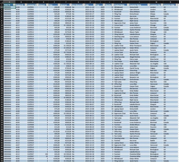3. Lesson 3 Getting Familiar With Excel: Start by getting familiar with Excel's layout. I use HachiPT to put the data together, and it's small enough that you can learn everything without getting overwhelmed. So the file that you have in front of you is called a workbook and each separate tab is called a worksheet. In this case, orders, product, customer data are all worksheets within the workbook. And this comes in handy when you start automating tasks using VBA Macros. At the top here, we have what is called the ribbon. This is the menu that holds most of your command options like formatting cells, inserting pivot tables, using filters, et cetera. And most of these commands have shortcuts. You don't need to memorize them all, but throughout the course, I'll show you the ones that I use the most. To be honest, I'm not a shortcut whiz, so I do use my mouse every now and then, but I try to limit the use as much as possible. This is because if you're using shortcuts, you will increase your speed and your productivity in Excel, when you're focused in on analyzing your data, you won't lose your thought process because you have to go to your mouse and then it just slows everything down. It's very important to know the main shortcuts and whatever you don't know, you can Google. Okay, moving on below the command ribbon are your grid lines. These are made up of a bunch of cells, and each cell is referenced by the column letter and the row number. So for example, order ID is in cell A one. And if you don't remember what the cell reference is, you can always check it out here at the top left where the cell reference will change as you move across the grid. You do want to get comfortable understanding the cell references because your functions will be using the cell references. So this is Excel's layout. The goal of this lesson is very simple. It was just to introduce you to the platform itself. So next we'll start with the heart of Excel, the functions and shortcuts so that you can start commanding the data to work for you. 4. Lesson 4 – Functions and Shortcuts: Now that you're comfortable with the platform itself, let's start with functions and shortcuts. A function is a command that tells Excel to perform a specific task, for example, adding up numbers or looking up values. All functions start with the equals sign, and there are mainly two kinds of functions aggregate and individual cell functions. Some of the most common aggregate functions are some average minimum, maximum. They give you a value based on your entire dataset. And when you're analyzing data and you're using pivot tables and lookups, you might not use these aggregate functions, but they are very useful when you have to give quick insights or if you have to present data in a meeting or if you have to use numbers to use in a presentation. That's when these functions come in handy, but you will mostly be using them when you're using your Excel sheet as a standalone item. So if we look at our dataset, the first aggregate function that I want to show you is the sum function. Like I mentioned before, to indicate to Excel that you're going to use a function, you start with hitting the equal sign and then you start typing in the function. If I write sum, you'll see that I get a bunch of different options, and as soon as I write the function, I have to open parentheses and then you'll see that Excel tells you the parameters that it's looking for. To get out of a function, you can just press the escape key, and I just want to show you a quicker way to type this in. You hit equals to indicate that this is a function, type in sum, and then you can hit the tab key on your keyboard. And it automatically comes up without you having to put in the parentheses. Now, this is where you will use cell references. What I want to do here is I want to add up the price of my first five items, and so I can just select my first five items and close parentheses and hit Enter. So you can see that the total for the first five items is 460. Now, every time you use a function and you come up with an aggregate value or any number for that matter, you should always ask yourself what that number means. Now, if I were to copy this number and put it in a presentation or send it to my manager, they wouldn't know what 460 is because there is no unit attached to this number. So again, whenever you see a number, you always want to ask yourself, what does this mean? In our case, this is the total price for the first five items, and so I want to add a unit to and I will add the dollar sign here, and now it is very clear that this is $1 value. Similarly, if I were to calculate the average of the first five items, I would hit the equal sign, start typing in my function and you can see that Excel pulls up different options. I will hit the tab key so that the function populates itself in the cell. And similar to the sum function, Excel will tell you the parameters that it's looking for for that function. Again, I'm going to select the first five items and close parentheses and hit Enter, and you can see that the average of the first five items is 92. What does this number mean? Is this number the total steps that you walk today or the number of apples that you bought from a store? 92 would be a lot, to be honest. But what is this number? What does it? This is an average price. So we'll go on this cell and click on the dollar sign. There are two more ways that you can format your cells in Excel. I'm just going to hit Command Z to undo the step that I just did. Under home, I can go to this option right here and select currency or accounting. And this brings up the dollar sign here. Another way to do it is to right click in the cell. Click on Format Sells. You can choose whatever category you want to pick. In this case, we can use either currency or accounting. I'll just go with currency and you can hit. Okay. Other common aggregate functions include minimum and maximum, and you can try that out yourself. In reality, you would use functions like some average to calculate your total revenue or your total profit or your average revenue for a specific month or a specific year. In this case, I just wanted to show you how to use the function itself. There are a lot of different ways that you can use multiple different functions. And if you have some ideas in your head, you can Google some functions and you can try it out yourself. One hand, where aggregate functions help you with the exploratory data analysis piece, which we will talk about later in the course, individual functions help you with the actual cleaning and analyzing part of your dataset. So let's get into that. A very common practice is to separate out the year and month from a date field so that you can look at trends over time, and this is where the year and month function these are individual cell functions, and even though this is not the first step that you will do in your analysis piece, I'm covering it right now because I really want to show you the difference between individual functions and aggregate functions and how to use different shortcuts and a few formatting tips that you want to use before you actually go into the analysis. So for this course, we'll apply functions before actually cleaning our dataset. Hit the equal sign, start typing in here. You can see that the option already pops up for you. I'll hit the tab key on my keyboard, and using the arrow key, I'll go to my date field. Close parentheses, and you'll see that we extracted the year from the date field. Now, if I want to drag and drop the formula, one option to do it with your mouse, which I don't really recommend and it really slows you down, but I want to show you regardless, is to hover over the bottom right part of your cell, and you'll see that the cursor changes a little bit. And this is your indication that you are ready to drag your formula to the bottom. I'm just going to drag the formula to the first instance of the blank cell that we have. So you'll see that the formula has been applied to all the cells. Command Z to go back. A quick way to do this using your keyboard is go to the closest column either left or right, whichever one is populated, and then hit the command end down arrow key. This will go to the very last cell before a blank cell. This could be because there are blanks in your dataset, or it takes you to the very bottom of your dataset. Then you can go back to the column that you want to drag the formulas down. You hit Command Shift and the upward arrow key, and it selects the entire range where you want to populate your cells with the formula, and you can hit Command Command D will drag your formula down to your entire selection. I want to do the same thing for the month. So how I can go back without using my mouse is hitting command in the upward arrow key, it goes to the very top of your sheet, in this case, we don't have any blanks, which is why it went to the very top. If you had blanks in your dataset, it would go to the first cell before a blank row. Equals, start typing in month, hit the tab key on your keyboard, go to the date column. And then close parentheses. Now, I'll go back to the closest column, hit command and the down arrow key to go to the last cell before a blank row or the end of the sheet, and then go back to the column that I'm interested in, Command shift, and then the upward arrow key to get the range of cells that I want to drag my formula down to and then hit Command D. So this is how you can apply functions and use shortcuts to populate your data set. Now, this was mainly to show you how to use quick shortcuts. But if you were actually applying formulas, the best practice is to convert your cells into a table, and I'll show you why. We'll convert our data cells to a table purely by using shortcuts. To select an entire column, you can hit the Control and Space key, and this will select your entire column. Then using Command Shift and the right AERO key, you can select all the columns that are populated that you want to convert to a table. And then to actually convert this dataset to a table, you can hit Command T, which selects the dataset that you will be converting to a table. And then if you hit Enter, you'll see that your dataset has now been converted to a table, and you can see that the table name here is table two. What I can do here is I can just call it orders. Now, going back to what we did before, I'm going to apply a function for year and month and you'll see that automatically Excel recognize that this is part of your analysis, and so it added another column to your table. So we can start typing in the function by hitting equals, and then I can type in, hit the tab key, select my cell, which is right next to it, where I want to extract the year, close parentheses and hit Enter. And now you'll see that the entire column is automatically populated and you do not have to do the work of dragging and dropping formulas. And this is why using a table is so important when you're analyzing your data, and this is going to be even more helpful when we start using pivot tables. As we move along this course, I'll introduce you to new functions that will be very helpful when you're going through the data analysis process. But now that you know the core functions and shortcuts, we'll move to the next lesson and explore how filters and blank rows impact data quality. 5. Lesson 5 – Filtering and Blank Rows: Now that we know the core functions and shortcuts, it's time to move on to filters and blancros because how you filter and structure your data determines the accuracy of everything that comes after. Filtering is important because it allows you to quickly find specific groups of data that share the same features. For example, all orders that were placed in year 2024 or all items that were returned. So you can quickly group things together, and there are two ways of applying a filter. The first is in the home tab under sort and filter. And the second way is to go in the data tab and click on filter. And you'll know that a filter has been applied when you see the arrows in the tiny boxes in the headers. Now, the way I applied a filter is not best practice because there are blanks in our dataset. You have to be very careful when it comes to blank rows, because in my demonstration, my dataset is very small. You can clearly see that Row 17 is a blank row with the exception of yes in the item return, which was clearly just a data entry flaw. But when you have large datasets, you might not know if there are blanks in your and if you simply apply a filter and start working on your dataset, you won't know that you aren't applying the same formulas to your entire dataset. Because when you simply click on filter, the filter is only applied to the first set of data before the blank Crow. So what you want to do, no matter how small your dataset is because you want to build the muscle of doing things right, you want to click on the arrow in the top left corner. And what this does, it selects your entire dataset. Another thing you could do is press Command A and then Command A again to select your entire sheet, and then you click on Filter. The filters will only apply to the active cells in your worksheet. In my case, I had some data in Columns INJ. I was testing something out. And so that's why the filters have applied on Columns INJ. Normally, when you select your entire dataset, the only columns that the filters will be applied to will be your active columns. Now, I could have added this as a quick pointer in one of my other videos, but I chose to keep this topic separate because of how important it is and how much grief it gave me in my early years of using Excel. I would have large data set when I was working at a construction startup. And I simply clicked on the filter. I did so much work and applied so many formulas on my dataset only to find out that I only did it on less than half of it because I couldn't see that there were blank rows. It really makes a difference, especially when you're sorting things, when you're filtering it all out. So the bigger your dataset is, the messier it can be. And so you want to build the muscles of doing things the right way so that no matter how small or large your dataset is, you'll always be sure that your data practices are accurate and that you're coming to the right conclusions and the right output. And for that reason, I'm going to quickly repeat what I said whenever you want to apply filters, you want to make sure that your entire dataset is selected. You can do that by pressing Command A twice or clicking on the arrow in the top left corner. Another shortcut is to press Control and Shift. To select your entire column, you can then click on Command Shift and the right arrow to select all the columns that are active, and then you can press Command Shift F to apply filters by using shortcuts. Once your filters have been applied, you can spot check some columns to make sure that your data is correct. For example, I can go into amount and see that I have a no in there. Because we will be covering data cleaning soon in one of the next videos, I won't do it right now, but filtering is a very good way to also spot check errors. All right, so now you have the basics down. You know where everything is in Excel. In the next lesson, we'll define a real problem statement to tie everything that we've learned so far together and see how logic guides analysis from start to finish. 6. Lesson 6 – Data Analytics Problem Statement: Now that we've learned how to use filters and clean up blank roads, let's move to the next most important step in data analysis, which is defining the problem statement. Whenever you get a dataset, whether it's for an interview assignment, a live case study or even your day to day work, the first thing you should do is ask the question, what exactly am I trying to solve? When I used to get technical interviews or Excel assessments, and then later when I was creating Excel assessments to interview other people, I noticed something very interesting. People jumped straight into the formulas, but the people who did really well always started by writing out what they were trying to achieve. Either in a textbox, a common, or a separate tab. You don't need to do this for your day to day work, but if you are doing an interview assessment, I highly recommend adding another tab called logical framework, and you can use it to outline your thought process, your assumptions, and your steps. Here's why this matters. It demonstrates your logical thinking even before you present your work to your interviewers, and this is what they're looking for, but barely ever. And the second is that if you forget a formula or syntax, your reasoning still shines through. So having a clear understanding of your problem statement and defining it before you start doing any work is going to be a game changer. For this course, we have three tabs, orders, product and customer data, and our problem statement is based on product performance and customer data, where is the company trying to expand next? And we'll try to answer this question by the end of the course. So now that we know what we're looking for, let's start exploring the data and see what stories it's trying to tell us. 7. Lesson 7 – Exploratory Data Analysis: There's a saying in data analysis that 80% of the work is cleaning and understanding the data and only 20% is analyzing. So before we build any charts or identify trends, let's start by exploring what's in front of us. Exploratory Data Analysis or EDA is you getting to know your dataset? You ask yourself questions like, What columns do I have? What does each one mean? Are the data types correct? Are there any missing values or weird patterns? So for example, if we look at the dataset in front of us, we can clearly see that there are some blank values in our dataset which could give us issues down the line. And so this is something that we will address in the cleaning part. I also want to see if there are other blanks in my dataset. So using filters that we learned in our previous lesson, I'll quickly see if there are any errors or blank cells. I'll pick any random column to look for that, and okay, so not only are there blanks in our dataset, but there is a random no in the amount column, which is clearly a data entry error because this column should only be accepting numbers, but there is a no in this column. So there are clearly some errors, but there are also blanks. So we'll address both in our cleaning piece. If your dataset is bigger and messier, you also want to make sure that the data types are correct because text cannot be added, right? So those are things that I would look at when I'm exploring my dataset. Another thing that we can look at is maybe age in our customer data tab. What I can quickly do is selecting the column, I can go into Insert and add a quick chart because charts are a really good tool to help you understand your data better. So here we can see that the age is 25-70, somewhere 25-70. But there's a clear spike where the value is 460. Now, this is an outlier and clearly an error. It's very normal to have outliers in your dataset, but you have to decide whether it makes sense to remove it or keep that outlier you don't want to remove true values from your dataset so it can look better. You want to remove the errors, like clear errors. So even in the blue zones of the world, nobody has lived up to the age of 460. So this is clearly a data entry error, and this is something that we will remove in the cleaning piece. Again, you want to make sure that you don't just remove all outliers because, for example, if we were only selling our products in the US, and you see that there is one product which is sold in Canada. Now, that could mean two things. Either that is an error or maybe our company is trying to expand in Canada and they have just started selling products. So if you just remove that one piece, that would be incorrect. In this case, however, this is clearly an error. So in our cleaning piece, again, we're just going to remove this. Is a benefit of the exploratory data analysis piece. You get familiar with your dataset, and you can get an idea of the work that is required in the next steps. The logic behind analysis always stays the same, no matter which tool you use Excel SQL, Python, you're always trying to convert raw numbers into meaningful insights. If you're using Excel to analyze any kind of data, dataset is probably manageable because for larger datasets, Python SQL are better tools, but Excel is still a very dominant software in industries like finance, consulting, accounting. And so it's very important that you also understand how to think and apply that thinking in Excel. The Excel project file is attached down below, and I hope that you're following along. For this project, our focus will be on expansion based on product performance, and that's the lens that we'll keep for the next few lessons. Next, we'll start cleaning our dataset, handling blank rows, trimming spaces, and removing duplicates to make sure that our analysis can stay as accurate as possible. 8. Lesson 8 – Data Cleaning: Now it's time for one of the most important parts, which is cleaning our data. You'll often get raw exports with inconsistent texts, duplicate entries, blank rows, and this is a process where you can start cleaning up those things. Like I mentioned earlier, I intentionally kept this dataset very small just so that you won't get overwhelmed, but we still look at the different aspects that you have to consider. You're cleaning your dataset. And I'll talk through my thinking whenever I'm looking at data. So first things first, we want to remove the blank rows from our dataset because like we talked about earlier, blank rows can cause a lot of problem, especially with filters, dragging formulas, stuff like that. So using filters, we can just select the blanks in our dataset. We want to delete the entire row and to do that, you can hold Shift and space, and it selects the entire row. And then holding Shift, use the down arrow key to select all the cells that you want to remove, and Command minus will allow you to delete these rows. Then we can remove the filter here. And before doing anything else, I want to convert my dataset into a table because like we saw before, it's very easy to drag formulas and just play around with different things when your dataset is in a table format because it removes a lot of the manual stuff that you might have to do. I'll select my dataset, Command shift, and the right arrow key, and then holding Command Shift, the down arrow key allows me to select my entire dataset, and I'm confident that this time it went down to the last row just because there are no blanks. In my dataset. So command, T, and Enter will convert this to a table. During the EDA process, I noticed that there were some inconsistencies in the amount column. I know that there is a text value which is no, and obviously, this is an incorrect value. This is a very good example for you to understand that knowing what your goal is for whatever task you're doing is very important. Now, if I wasn't analyzing my data to understand where I can expand my company based on product performance, I would have taken a very different approach. If I was just collecting data and making sure that my data was complete, I would go back and look for the order ID in whatever software I'm collecting all of this information or if I have a database, I would go there and make sure that I know the amount of items that were bought in this order in order 68. The reason that this is clearly a data entry issue because there was a no that was added. There should have been a number. And this clearly looks like it was an export from another platform where we're collecting our order data. So I would go into that platform and replace the no with the actual amount because I want to make sure that I'm not losing any of my values. In our case, we don't really have access to the platform where all of the orders were gathered. And so, obviously, we cannot replace this value. What I'm going to do is I'm just going to go ahead and delete this from my dataset. But I just wanted to make the point that it's important for you to understand what you're doing more so than just doing the steps because your decisions might change based on the task. So I'll select this line item using shift in space and Command minus. Enter to remove this. Now I'm going to quickly check that everything else looks fine. There's nothing in the price, item returned is also just yes and no, so everything else looks great. One thing I want to do is calculate the revenue. You can do this in the next step or later, but I would prefer doing it right now while I'm cleaning my dataset because I know that everything is clean right now, and I also know what my goal is. So revenue is an important metric that I would want. So what I can do is I can add a column here. Right before items return and after amount price, I can rename this called this revenue, and revenue is equals to start a function. It's amount times price to give the total amount. Now, if this weren't a table, we would also have to drag drop our formulas, but this is because our data is in a table format, we don't have to do that. Now, amount, price and revenue, it seems like, has the same data type, but there are two very different items. Amount is just the amount of things that a customer has bought, and price and revenue are dollar figures. So I want to change that because I want to be very familiar with my dataset, and I really want to understand what the different data types are because the calculations that I will perform will be based on data types. Sometimes what happens, actually, most of the time, when you're exporting your data, the data types might be incorrect. So you might get numerical values in text formats. What that does is that it doesn't allow you to perform specific operations like some average multiplication division on text because obviously, it's not a numerical value. So you want to make sure that your data type is always correct so that you can perform all the different mathematical operations that you would want to do based on whatever you're calculating. In this case, I will select the two columns and then convert them into dollar values. You can see the hashtags or the number signs. I don't know what this symbol is called. I call it hashtag, but it just means that the width of your column isn't enough to fully display the number here. So you can hover over that particular column where you can see the the line and the two arrows, and you can double click on that column and it'll fully expand to show you the entire number. And then the number or the hash sign will be removed. Another thing is I want to extract the month from the date field, and using the month function, I can extract the month. So I'll start typing in the function, hit tab and go into the date field, close parentheses and enter, and we'll see that now our column has been populated with all the months. Okay, next, I'm in the product tab. And what I want to do here is I just want to look for duplicates because maybe during the data entry process, we added multiple items. And this is also a spot check to make sure that there were no incorrect items added or incorrect price or maybe we have the same product ID, stuff like that. This is where I'm going to look for that part. So selecting the entire column under home, I'll go into conditional formatting and select duplicate values. And then hit Okay. So I can see that I have two duplicates. One is a whiteboard and both are white, both are $100. So this was just an entry that was added by mistake. And so I'll just command minus remove or delete this column. The next duplicate item is A 112. Now, this is an error because the same ID is referencing two different products. One is a green for trust and the other is a black for trust. For our case, I'll assume that this was an incorrect entry, and I'll just go ahead and remove this duplicate value as well. Right, so now that we don't have any duplicates, I'm going to go into the last tab, which is our customer data. Instantly, I can see that there are some extra spaces in the name columns, which is not good. Spaces can be a huge issue when it comes to looking up values because when you're looking up values using V Lou index match or lookup, which we will be covering in the next parts of the course, the lookups are sensitive to characters. Any extra character, a space is a character, a letter is a character, a comma is a character. Lou can get confused about what you're trying to pull and it won't pull the same thing. So Liam Johnson in Cell two is different from SpaceSpace Liam Johnson. For that reason, we have to make sure that we don't have any extra incorrect spaces in our dataset. Another thing that I want to do is I want to combine first name and last name into one, so I will use the concat function, and you will probably be using this function a lot, especially with something like this. If you're collecting data from customers, it's very common to ask for the first name and last name separately. But for the dataset, it's very helpful having the full customer name, even though you would never be using the customer name as a lookup function. As a lookup value, sorry, you will either use the customer email or a customer ID because that is a true unique value always. So first, I'm going to bring these two together using the concatenate function. Before I do that, I want to convert this to a table to make life easy for me. And now I can add another column, call it customer name, and using the concat function, I'll bring these two together. I can start a function by hitting the equal sign. Concat, you can see that it already comes up, hit tab. Now, Concat takes different texts as parameters, as you can see in the function help box right below, and it considers every single character. So in this case, we'll use Emma and then then we need a space between the first name and the last name, so we have to specify the space as well, and last name. Close parentheses, and we can see that the formula has been dragged to the very end, but we still have extra spaces that we don't want. So I can now use another function to remove the extra spaces, which is the trim function. The trim function can help you remove all extra spaces and then close parentheses and hit Enter, so we can see that all the extra spaces are now removed. Now that we don't need our customer name, I can just go ahead and delete it and you'll see something interesting that happens. So I can see that as soon as I remove the customer name column, I get a reference error because the cell here has a formula which is attached to the column that we just deleted. And so it doesn't know where to reference anymore. And this is very important when you're working with different workbooks, especially if you're building up an Excel sheet to send to somebody else, if they don't have access to all the worksheets or all the workbooks that you have referenced, In your final worksheet, they will see the reference errors. So it's extremely important that you convert these into values and don't keep these things as formulas. In our previous stab in the order Stab, I don't have to do this with revenue because I know that amount and price will always be there, and they're in the same worksheet. But in this case, in the customer data tab, we're using a column that we're not going to need. And so if I go back hitting Command Z, now we have the customer name formula there. And what I'm going to do is I'll command shift and down okey to select the entire column. I'll copy and right click Paste Values. Now I can see that it no longer is a formula here. It has pasted all the values. Now if I delete this column, you'll see that nothing happens and our dataset is fine. It doesn't go crazy because it's no longer referencing another column. So I can change this to customer name. And honestly, I don't even need the first name and last name, so I can just delete this. Next thing I want to do is address the outlier in our age column. We decided in the EDA phase that this is something that we will remove from our dataset. Again, you don't remove all outliers. You have to really understand what that outlier is. In our case, this is an incorrect value for sure because nobody can live up to the age of 460. Maybe there's some technological advancement that happens in the future. But now, as of today, no one can live up to 460. Even in the blue zones, the max that someone has lived is, I think, 120 years or something. So this is clear error, and for that reason, I'm going to remove it from our dataset. If I thought that this was something that was an actual outlier based on the data that we have entered or the data that we have collected, then you will not remove this. All outliers are not removed from your dataset. Only the ones that are clear errors are removed. So shift space to select and then command minus, okay? And now I can clear the filters. This process wasn't very difficult because our dataset is pretty small and quite clean, actually, for big data standards. This is not even considered close to big data, but data can be very, very messy. But the overall approach stays the same. You're always looking for duplicate values for incorrect data types, for blank rows. Those are the main things that you will look for. You'll address outliers, stuff like that. So we've covered the majority of the things that you would need to know when you're cleaning your dataset. But obviously, the bigger the data is, the more messier it can. Leaning does take time, and you might get impatient because you want to do the fancy stuff right away. But just remember what I said before that data analysis is 80% understanding, cleaning, exploring the data, and only 20% analysis. And if you spend time cleaning the data and understanding the data, you'll be very happy with yourself when you have to do the other stuff. Now that our data is clean, we can start connecting different sheets and bringing everything together using lookups. And the first lookup that we will use is V Lookup. 9. Lesson 9 VLookup: Now that our data is clean and ready to be used, it's time to talk about one of the most useful and powerful functions in Excel, which are lookup functions. Look up functions allow you to connect information across multiple sheets and workbooks, for example, connecting product IDs to actual product information, customer IDs to actual customer information, and they help you organize and bring your data together in a way that your analysis is seamless and more accurate. In this course, we'll talk about three lookup functions. The first is V Lou which is the classic and easiest one to understand. Second index match, which is more flexible and powerful than Vu. And the third is lookup, which is the modern all in one most powerful, most flexible lookup function which is available in newer versions of Excel. Starting with V lookup, it's short for vertical lookup, which means it looks for a value vertically until it finds a match. Typing the function here, you'll see that V lookup requires three mandatory parameters. The first is the lookup value, which is the value that you are using to look up another value the table array is where your final value lies, and the column index number is the number of the column where your data is in. So these are the three things that you have to enter for Lookup to work. So using it in our dataset, let's look through the different tabs to see what information we will be using. Here we have order ID, product ID, and customer ID. So let's first go into the product tab. We can see that in the product tab, we have the product name and the product color and the unit price. I believe we already have the price yes, we already have the price, so we don't need to bring that in from the product tab, but we don't have the name of the product. We only have the product ID, and to make our analysis better, we want all our information from all three tabs combined in one tab. So we're going to bring data in from the product and customer data tabs into the Orders tab. So the first thing that we want is the product name. We'll start by typing in the function. The first parameter is the lookup value. This is the value that we will use to look up another item. We're going to use the product ID, which is the lookup value to look for the name of the product. So in our case, our lookup value is product ID a 108. And then once we've added the parameter, it's time to add the next parameter, you hit comma, and now it's asking for the table array. Now, this is the table that both our lookup value and our final value lie in because we will be using that particular table array to get the information. So our table array is obviously the product tab, and these are the four columns that we will be using for our table array. Now, the important thing for V lookup is that our lookup value, which is the product ID, has to be in the leftmost column. If it's not in the left most column or at least to the left of the column that we are interested in, it won't work. So because product name is what we want, we want to make sure that product ID, which is our lookup value is on the left. In this case, it is. So we will hit comma again and now it's asking for the column index number. So starting from the left and including the look up column, we'll start counting. So A is number one, and B is number two. And because product name is what we're looking for, we're going to put in two and close parentheses and hit Enter. And then you'll see that automatically it dragged the formula all the way down because this is a table. Now, the reason that I don't like V Lou and the reason why I don't use it unless I have a very small dataset, and I just want to quickly get information, and I know that I'm never going to look at it again is because it's not flexible at all. In this case, our dataset is so tiny that it doesn't matter what kind of lookup function we're using. Our product ID is to the left. It's just the perfect case scenario, but that's not always the case. If our product ID was somewhere in between and we have lots of different and we had lots of different information, it would take so long for us to arrange our dataset first to make sure that our lookup value was to the left would just be a waste of time. Another issue is that if our dataset is changing in any way, it can break the function. For example, if I were to add an extra column before product name, you'll see that now our V lookup function no longer works because it's looking for column two. Column two is empty now, and so it's not pulling anything. So it's not flexible and it's not dynamic, which is why I'm not really a fan of V but I also see that it can be very helpful if you have a very small dataset and maybe you're building a presentation and you quickly want some answers and you don't care if more columns are inserted, deleted, you don't care about that, then V Loup is perfect. So going back if I delete this column or if I just hit Control Z, you'll see that now the formula works fine. Loup is extremely simple. Make sure that you're working along using the project file with me because it really helps to strengthen your concepts. So we talked about the pros and cons of Lookup, but when you have larger datasets, you would want more flexibility and would need a more powerful function for that purpose, and this is where Index Match comes in. So in the next lesson, we'll see how Index Match gives you more control over your dataset. 10. Lesson 10 Index Match: Now that we've talked about Lou, let's move on to the next function, which is Index Match. Index Match used to be my personal favorite combo because it's both flexible and powerful and we'll talk about why my preferences have changed in a few minutes. Unlike V Lou, which only pulls data to the right of the lookup value, Index Match can pull data from any direction, and it does not break if you make any column changes. Back in 2016, when I was working at the Construction startup, I learned index match by going through a whole paragraph of different functions and breaking it down one by one to see what each one means, and that's how I learned this function. Nested functions can feel a little complicated, but they're really not, and they give you a very good understanding of how overall functions work in Excel. So we'll start with the match function first. For this function, we'll be pulling in the customer name from our customer data tab using customer ID as the lookup value. So let's write customer name over here, and we're just using the match function first so that you know what the match function returns. Equals match and you can hit tab so that it populates. It's asking for two mandatory parameters, the lookup value and the lookup array. So the lookup value will be the ID which we will use to pull the customer name, and the lookup array is the column where the ID lies. So customer one is our lookup value. And if we go into the customer data tab, our column A is where the customer ID lies. And then close parenthesis hit Enter. So the match function return numbers, what does this mean? Customer 001 returned two. So if we go into the customer data tab, we can see that customer 001 is in the second row. Let's look at a few mores. Go back into orders, and customer nine returned nine. If we go into customer data, customer nine is in the ninth row. So this means that the function match is returning the row numbers where your lookup value is. Now that we know what the match function does, let's move on to index equals index, and then you can hit Tab, it's asking for two mandatory parameters. The first is the array, and this is where our final value lies. So in our case, it's a customer name in the customer data tab. Then it's asking for the row number, which if you remember, we got from the match function. So instead of adding a row number, we're going to use the match function to grab the row number for us. So let's go into customer data. And then select customer name as the column that we want, now it's asking for the row number. And if you remember that we used the match function to grab the row number for us, so we won't be doing this manually. We'll use the match function here so that it can grab the row number for us. If I type in match, then it's asking for a lookup value, go into orders and grab customer ID because we want customer information, and customer ID is the primary key in the customer data tab. And it's asking for the lookup array. Where is the customer ID under the customer ID column. One thing I forgot to mention when I was showing you the match function is you have to specify whether it's an exact match or not. So we can do that by hitting and zero, which shows that it's an exact match. You close the parentheses, and now this has closed the match function. So when you close the parentheses, now our match function, it's indicating to the function that match is closed, and now you'll close the index function by adding another parenthesis at the end. Hit Enter and you'll see that the customer name has been added. I am not sure why this is an NA, customer 005, customer 00o. See, there is no customer 005, which is why it's giving us an NA. I'm not sure where this information came from. Maybe when I was cleaning up the dataset, this could have been the 460-year-old person that we removed from our dataset. So what I can do is shift space to select and command minus remove this from our dataset. Again, if you were doing this in real life, you would go back to the software or whatever platform, gather your data and look up the information and see if you can grab the original data to put into your dataset. And sometimes it's just an error, so you can remove it from your dataset if it's an error. But by default, don't just assume that if something is missing, it's an error or if something is an outlier, it's an error. That's not always the case. So you saw how the index match function works because it's more complicated than Vu, we'll do another one and make sure that you're following along in your project file. So now what I want is the city. I can just type in customer city, and I'll start with typing in the index function hit tab so that it populates. It's asking for the array, the final array where your destination lies. The value that you're looking for, where does it lie? It's in the customer data tab, and it's in the city column because we're looking for the city. Asking for the row number. This is where we'll use our match function. We need the lookup value, which is in the orders tab. Obviously, it's the first lookup value because this is an individual function and we want it to apply to all the values. It's not an aggregate function. It's asking for the lookup array. The lookup array is our lookup value, like where our lookup value is, which is in the customer ID column. We want an exact match. Close the match function with the first parenthesis and then close the second function with the second parenthesis. Hit Enter, and now we have the city for all our customers. Whenever you're doing lookups, you want to do quick spot checks. So what I'll do is I'll just make sure that the information is correct. Customer 002 is in London, which is correct. Now the way this function is set up, it doesn't matter where your ID column or your lookup column is because it can be anywhere since you're just selecting the column and you're specifying where your lookup value is. The function won't break if it's on the left or the right. And the second issue that we had with Vlookup was if you inserted or deleted any columns, your function would break. So let's test that out as well. If I go into customer data, customer name was one of the values that we pulled. So if I insert a column over here, and go back to orders. So you'll see that the column did not break, and that's one of the flexibilities that Index Match offers you, which we look up does not. There are two main disadvantages with the index match function. One is that it's slightly complex and so difficult to write. But if you practice enough, you can easily solve that issue. And the second is that if there are any errors or if there are any missing IDs in your dataset, it won't return anything. So if you remember, when we had customer 005, adding that back again, customer CST 005, we got an NA. Obviously, there's no ID, so it's giving you an error. But if you want to specify what to do if there is an error, you have to use the if error function, and you can say not found. And close parentheses. So I basically added another function called if error, and then I specified what I would want if there was an error. Let me do that again. So I basically go in here and I write if error, which is another function, hit tab for it to populate itself, it automatically adds the first parentheses and the two values that it requires sorry, the two parameters that it requires is the value, which is what we're getting from the index match function. And then it's asking what happens if the value that is returned is an error? So you can hit comma, so it goes to the second parameter. And then you can maybe type in not found. Close parentheses and hit Enter. So if there is no value that is found, then you can say not found, but you have to use another function for that. So that is the second disadvantage of the index match function. But there is another lookup function called X Lou, which solves all the problems of V Lou and all the problems of index match and combines it together in a new, more flexible, more powerful function. So now that we understand the concept and we know the more complicated version of lookups, let's move on to X lookup. 11. Lesson 11 XLookup: We've looked at V Lou and Index Match. Now let's look at the newest, most powerful lookup function in Excel, which is X Lou. X Lou was designed to fix all the limitations of V lookup and index match while keeping the formula short and simple. Before we look at what X Lookup does, I'm just going to hide some columns so that you can see it clearly and it becomes easier for me to edit later. All right, perfect. So we'll be using Xo up to pull up customer country. From the customer data tab. Typing the X lookup function, we can see that it requires four mandatory parameters. The first is the lookup value, which in this case is the customer ID because using the customer ID will extract the customer country from the customer data tab. The second is the lookup array. So where is this lookup value in the dataset? The third is the return array, which is the data that we are actually interested in, in this case, customer country. And the fourth, actually, this is not a mandatory parameter because we can see that it's in brackets. It's an optional parameter, but it's the if not found parameters, similar to the I error function that we used in the index match function. So using the four parameters, we're going to see how X lookup works. Our lookup value is the customer ID, so customer 001, to go to the next parameter, our lookup array is in customer data. Look up array is basically where is the lookup value, and the lookup value is somewhere in the customer ID column. The return array is what we're interested in. In this case, we're interested in the customer country, and we can also add an if not found optional parameter, which is if we don't find the particular customer ID that we're looking for, we want our function to return not found. Close parameters and we hit Enter. You can see we get all the values for the different customer IDs in seconds, there were no nested functions. We don't care if the columns move here and there. We can also test that out. So if I insert another column anywhere in my dataset so that the columns move to the right, we'll see that our function did not break and we still have all the values that we are interested in. Now, we don't have customer 005, which initially gave us the error. So let me add it in to show you how this works. Insert and customer 005. So we can see that instead of NA, which we can see in columns L and M, this function without adding an extra function is giving us not found. So if you have a very large dataset, you can really use this function to your benefit because you can very simply, without adding an extra function, specify the value that the function should return if the lookup is not in your dataset, and then you can filter or look at it in pivot tables. It's very easy to see which values you do not have. So this is one of the main things that X lookup provides, so the other functions do not I would again encourage you to try this function out yourself in the project file because no matter how easy this looks, you will get confused. If you don't practice it yourself. You really have to understand the lookup values, the primary keys, and the return arrays to really get some benefit from lookup functions. So this is why X Loup is my new favorite lookup function, and initially, I didn't really know much about it because I was used to using Index Match since 2016, and X lookup wasn't a thing at the time, which is one of the disadvantages of X Loup that if you're using an older version of Excel, this lookup function will not work. And if you're working on an Excel file on your computer and it's the newer version of Excel, but you send it to somebody who does not have that new version installed, then this lookup function will not work and they'll only see errors. So if you are sending it to somebody, if you are sending the file and you're sending it to someone who you know has an Excel version which is updated, then using this function is amazing. But if not, I would encourage you either to use Index Match or to convert your formula into values like we practiced in one of the previous classes so that you can be sure that your function will not break, and whoever is reading your Excel file will have all the values that you want them to see. We've covered all three lookup functions, and we used V Loup, Index Match, and X Lookup to bring our dataset together into one tab. Now it's time to take this clean connected data and start analyzing it using pivot tables, which is one of the strongest features in Excel. And the next lesson we'll build Pivot table step by step to summarize data, identify trends, and bring our project together visually. 12. Lesson 12 Apply Logic Using Pivot Tables & Charts: Now that our data is clean and connected, it's finally time to work with one of the most important features in Excel, which are pivot tables. If you've ever needed to summarize large amounts of data, this is how you do it. Pivot tables can help you find insights, trends, and answers without writing complex formulas. And honestly, if you have to do any kind of analysis in Excel, you must know how to use pivot tables. Alright, so we've already converted our range of cells into a table, and there are two main reasons why you would want to do that. First one, I think, is more of a Windows problem than it is a MAC problem, but the problem is that if you don't have a header, for example, if there was no header in items returned, if this was just a range of cells, you would just see that the header is removed. In that case, if you try adding a pivot table with that column included, it won't work. I'll give you an so you have to make sure that all your columns have headers. And honestly, I don't really mind that problem a lot because it is nice, especially when you have large amounts of data to have headers in all your columns, otherwise, you can get lost. So that is a good problem, in my opinion. The second issue is that if you start getting additional rows in your dataset, you would have to change the selected data range again and again to make sure that you're all of your cells that you want included in your pivot table. However, if you use a table, that won't be the case. So that is a big benefit of using a table when you're creating pivot tables instead of just a simple range of cells. We know that our data is in table format because we can see the table option in the ribbon at the top, and you'll notice that as soon as we insert a pivot table, that option will appear as well. Let's change the name of the table here and call it orders, so it's easier for us to navigate through the different tables. When you have multiple tables, you'll see why doing this is really important. Let's go ahead and insert a pivot table. You don't have to select the range of cells because we already have everything in table format. But if this was just a range of cells and not a table, you would have to select your dataset. And then insert a pivot table. If you just select the entire dataset, you'll see that your pivot table has a lot of blanks, and that's not really fun to see. It messes up the analysis, and actual blanks can be ignored. As a result. You don't want to do that. And so you only will select the range of cells that you want included in a pivot table. In our case, we don't need to worry about that because our data is in a table format. Insert pivot table I like adding it in a new worksheet. If I was creating multiple pivot tables for the same table, then I would keep those in the same worksheet. But the first pivot table you can create in a new worksheet and then hit Okay. Alright, so we now have a new worksheet with the pivot table options in front of us. So on the right, we have the pivot table fields panel, and this is where you have all the different options for rows, filters, columns, and values, you can simply drag and drop your selected field into one of these boxes, or in a MAC, you can just click on the field name that you're interested in, and it automatically assigns itself. You might want to change that depending on what you're looking for in a table, and it's not always accurate. So I like adding it myself, and you can simply drag and drop it's super easy. So the question that we want to answer is, where should we expand based on product performance? And for that, the first thing I want to see is total revenue by country. So let's go in and select customer Country. You notice that I simply clicked on customer Country and it appeared in the rose. That's where the first option will always appear. And if I were to select any other option, it keeps going into the rose field, right? So to remove a field from one of the boxes, you can just click on that field and remove it out and it disappears. So this is the total revenue by country. So as we can see that there is a not found option in our pivot tables, which is incorrect. This is one of the things that I really like about pivot tables. If you miss something in the filters, you will see it instantly as soon as you insert a pivot table. So clearly, there is an issue in the customer country. I imagine that it might have got something to do with customer five or maybe something that we removed from our dataset. So we can go into orders and using our filters. All right. So we can see that there is a not found option here. So yes, this is for customer five, and like we did before, we can simply remove this field from our dataset. Like we mentioned before, if you were doing this in real life and you had another platform where you were pulling data from, you would want to go back there and make sure that you don't have any information connected to customer five because if you do, I would rather that you pull that information and get your dataset completed instead of just simply deleting for our purposes, our dataset is small and obviously we don't have any other platforms because this is a chat GBT generated dataset. So I'm simply deleting the rope. But in real life, you don't want to just delete data, be it outliers or missing data, you want to first go and see if you can actually collect the data, and then for outliers, you want to see if you can understand the reasoning behind an outlier. And then you want to decide if a data point should be deleted or not from your dataset. So shift space to select the entire column and then command minus we do want to delete the entire sheet row, and then you can clear the filters, go back up using the command and upward error key. All right, so if you go back into our sheet one. So the not found option is still there, which is a problem. We just removed it, right? But in pivot tables, you have to manually refresh your dataset every time you make a change. So if you go into Pivot Table, analyze the option here to refresh can be selected. And now we can see that not found is no longer a problem. Coming back to our question, which is, where should we expand based on product performance? We would have to go through a few layers of data to understand where we should be expanding. So from a quick look, we can see that UK has been our best performing country in terms of revenue. In this class, we're only looking at the total revenue to decide if we want to expand to another country or another city or not. But in real life, you will never just use one data point to make such a big decision, especially if you're interviewing for consulting roles or if you are a consultant, you'll know that just using one field is a recipe for disaster. And I have been emphasizing outliers and deleting datasets and not using one field because it's extremely important in data analytics that you use your thinking and your logic to make decisions, any decision, whether it's deleting a dataset or just deciding on one data point, that's why I'm emphasizing that over and over again. So if we just have the total revenue, we are never going to make the decision of expanding into a new country because there are so many different factors, tariffs, unemployment rates, the different laws in a country, whether it's actually easy for us to expand or not. What are the other expenses for country one versus country two? These are many factors that you would have to consider when you are making a decision for any problem that you are trying to solve using data. The qualitative aspects are as important, if not more, as the quantitative aspects any problem that you are solving. So that is something that you have to keep in mind whenever you're looking at numbers. So we have the amount, which is the total revenue. In this case, it's very obvious that UK is number one. But if you had multiple different entries, you wouldn't want to see the relative performance of one country versus another. To do that, I would pull in revenue again in the values field, right click the sum of revenue options and go into field settings to show data as a percentage of the grand total and then press Okay, because percentage gives you relative information. Dollar values are giving you static information. And so when you have a lot of different options, you really want to see how one option works versus another. And when you have multiple options, it's very hard to compare one option versus another. So in this case, we know that 65% of our products are being sold in the UK and 20% are being sold in Canada. So UK might seem like the obvious option, but we're not going to make that decision right away. We have other things to look at, as well. So now that we have an idea of relative performance, I can just remove the sum of revenue option. From the pivot table fields panel. And the next thing that I want to see is the performance year over year. I'll pull the year field into the columns section. So we can now see the performance 2022-2025. So 22-23, the revenue in Canada was slightly increasing, but UK was a massive increase. But then since then it's been declining. But our revenue in Canada in 2025 is a lot higher than UK or the USA. So I can say that both Canada and UK might be valid options to compare against. And again, we have to consider that this is randomized hatchbT data, so it may not be as accurate as the data you would actually get for sales in different countries. In a real data set, the trends that you would see would be very different from what you're seeing here right now. So the decision that we might have to make is between UK and Canada at the moment. USA is not a contender because the revenue numbers are very low, and even though we won't be basing our decision just on revenue, it is a very important factor. So if that factor is not even something that we would consider for USA, we can just eliminate that option right away. So now that we have a year over year idea, we can just remove year from our columns. And now I want to look at product performance. I can simply select product name and place that under customer country in the rose section. And now we have the breakdown by product. Again, total revenue is not enough information to understand how many products we actually sold and how popular product is because, for example, if bookshelf cost $1,400, that means we only sold one of that product. Want to understand the volume of the products that we are selling. And for that, we can just pull an amount and I actually want amount on top of revenue in the values section. All right, so I'd like to sort my data so it's visually pleasing. I can go into the filter up here that you can see, and the field that I would like is, I think, customer country, and I want to sort by total revenue, descending. So now we can see that UK is at the top, because obviously the total revenue is the highest in the UK. I'm also going to sort by sum of amount in descending order. And now I can see that footrest is what we sold the most. The total amount sold is 160 footrest products, which is quite a lot compared to all the other products that we have. So from this data, we got some understanding of what is working in which country. So Futrust is working the most in the UK. 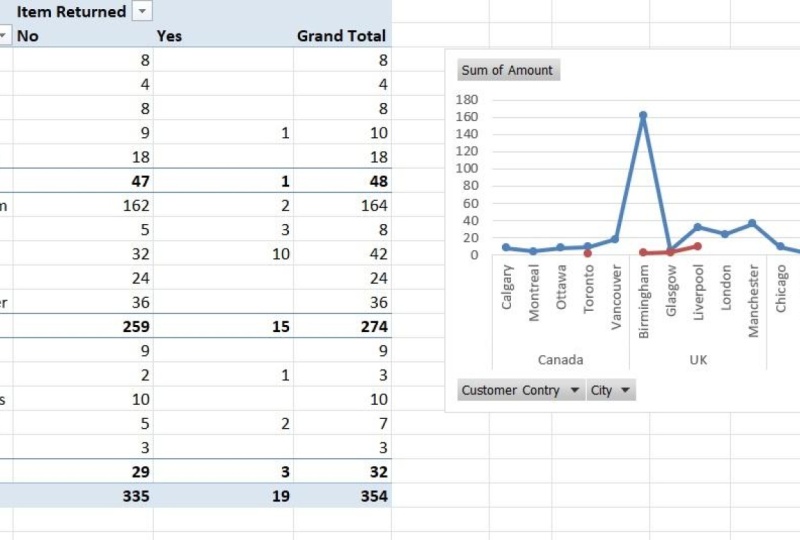Our expansion decision will obviously be different based on whether we have an online store or a brick and mortar, but this data at least is giving us an understanding of which country is the most now that we know which country is the most favorable, I can shortlist my options to the UK. And now we can check which city is the most favorable so that we know where we want to open up a new store. So what I can do is remove the product name because now that is no longer relevant, and I can look for customer city and bring that under the customer country option. Because I'm not really looking at Canada and the USA, I can just collapse those fields. So we're only looking at UK. And from our data, we can see that Birmingham is the place where we might want to open up a new store only based on the number of items sold and the total revenue. Again, I want to emphasize that this is not our final decision for the data that we have and for our case, it is our final decision, but in real life, there would be a lot of different options that you would have to consider before making a decision. Another quick thing that I want to show you about pivot tables is you saw how important pivot tables are, right? The numbers are great and you got a very quick understanding of what works, what doesn't work. Numbers are always better when you can visualize it, and this is where pivot charts come in. Pivot charts can assist you in your analysis because you can quickly insert charts, and they keep changing as you're changing your pivot table if you're just using your pivot tables to get an understanding. So, for example, we started off with customer country, and then we looked at product performance, and then we narrowed it down to the cities. To view a pivot chart, you would simply make sure that you're in the pivot table analyze section. And to the right here, there is an option for pivot chart that you can click, and you get a quick visualization that UK is your highest performing country. Again, this is more useful when you have different options and you want to see quick answers. So if I were to drag customer city, in the rose column, you'll see that the pivot chart has automatically been updated based on the selections that we have in our pivot table. So if I were to expand Canada, you get the different cities in Canada, and if I were to expand the US, then you have all the different options here as well. Obviously, this can get a little confusing the more charts that are added. But the good thing about pivot charts is that you can visualize your data as you're trying to analyze it. So if I'm just looking at UK, I can simply collapse Canada and USA options. So now I just have the view of one country. So you can play around with pivot charts as you wish, but it really helps you to visualize your data as you go. This can also be very helpful when you want to add charts to a presentation. And as you're analyzing your data, you can keep gathering the different charts to really visualize the experience for other people who will see it's very important that you choose the things that you want to show based on the audience. So if you're presenting to senior management, you will use different charts and more concise overarching theme charts. But if you're presenting to a specific team who would need more data, then you might want to present the pivot table, which has the nitty gritty of each data point rather than a chart that only shows overarching themes. So based on your goal and the audience that you are presenting to, your method of presentation will also change. So make sure you keep that in mind as you're going through your datasets. Speaking about logic and understanding, one thing I want to mention that if this were an interview, you could also add a tab called logical framework. And here you can just outline the different steps that you've taken to analyze your data or your thinking and logic behind whatever you've done. This way, you're helping whoever is looking at your work to go through your thoughts and they don't have to play around the data themselves. And sometimes there are things that you might be thinking of and you might be considering that other people don't know that you are considering for example, when we talked about revenue and not only considering revenue and making an expansion decision, this is something that you can add in your logical framework field because if this was your regular day to day work, you could have that discussion with your manager or with your team. But in an interview setting, you might not be able to do that because many times companies give you technical assessments, and if they like your technical assessments, then they move you on to the next round, which is the presentation of the case study. So having a logical framework tab will always work in your favor, especially if you're understanding solid. Now you know how to bring your data to life and use simple numbers to understand a bigger problem. 13. Lesson 13 Conclusion: And that's it. You've made it to the end of the course. We started with the basics, learned how to logically think about data, cleaned and prepared our dataset, applied lookup functions, built pivot tables, and finally visualized our data using pivot charts. If you followed step by step, you now know not only how to use Excel, but how to think like an analyst, and that is what's going to set you apart. Remember this, anyone can apply formulas. It really is very easy to do so. What employers are looking for and what will make you stand out at work or in your personal business is how you think about data and how you find the why behind the numbers and communicate it clearly. Thank you so much for taking this course. Keep practicing, keep experimenting. Always start with logic before formulas and happy analyzing. Bye.