Transcripts
1. Introduction: Self-driving cars, augmented reality, voice assistants. These are products of the near future enabled by artificial intelligence. Ask how artificial intelligence works though, and you'll get a bunch of deep neural things, graphs, figures, visualizations, memes even. Confusing. This class is different. I'll explain what's going on behind the scenes with substance, without intimidation. Not using buzzwords just for the sake of it. This time, you are learning machine learning for real. Hi. I'm Alvin. I'm a Computer Science PhD Student and Lecturer at UC Berkeley where I've taught over 5,000 students. I've worked on deep learning research for production-facing applications. First, for two years at Facebook Reality Labs and Mixed Reality for products like Oculus Quest. Now, at Tesla Autopilot for full self-driving. Based off of years of production facing research, I'm distilling machine learning concepts into a practical introduction for you. This class is written for anyone intrigued by artificial intelligence and machine learning. Believe it or not, the secret is to take a step back and learn the foundations from ground zero to break down a sexy AI product into its component and all parts. Taking this course, you're taking a meaningful step towards applying ML towards your product, your hobby, or your business. You can be a coder or a completely non-technical person of business leader and artist; anyone really. However, if you don't already know Python, you'll get a lot more from the course by taking my Coding 101: Python for Beginners course. For everyone; coder or not, the primary goal of this course is to build a foundation for your future machine learning education. This means; one, learning how to learn machine learning, and two, applying this method to learning a few introductory concepts. To succeed as an ML practitioner, you need code and math. We'll work on both of these in this course. In particular, we'll cover fundamental math concepts and terms as it applies to ML. Don't worry, no funky Greek symbols. Just the ideas. How to use a popular machine learning library in Python? We'll then use this to build a face and motion classifier, and finally, knowing the vocabulary for machine learning so that you can talk comfortably about ML topics. We're striving for understanding of core ML concepts, not just stuffing deep learning something into every single sentence. That can be for our future course. In this course, we're learning the fundamentals. Understanding machine learning will go a long way. After taking this course, you'll have the tools, the vocabulary, the knowledge to begin learning about other machine learning fields: computer vision, natural language processing, you name it. Understand the applications of deep learning to that field, but first we're going to learn the foundations of machine learning the right way in this course. Let's get started.
2. Project: Your project in this course is to break down a machine learning problem that you find exciting into its component parts. We'll cover these component parts, data, model, objective, and algorithm in lesson 3. This will help bolster your understanding of a fast-moving AI ML world. As an example of breaking down a problem along with code, you'll build a face emotion classifier. Don't worry, no coding experience is required. If you don't already know coding, you can simply copy each line that I explain and write. However, you'll get more to the course by understanding Python. You can get caught up by taking my Coding 101, Python for beginners course. This face immersion classifier is a great way to see one, ML concepts in action, and two, a visual way to understand the power of ML. This is one of my favorite parts of computer vision. The fact that you can see your ML model working, and maybe most importantly, it's critical to see that even the simplest of ML models can be highly practical. If you can produce a quick and easy ML solution in just minutes, you absolutely should. All it takes is the insights and the fundamentals that you'll pick up in this course. Sometimes you don't need a fancy model and sometimes you do. One, we'll start with the big picture, what AI is, what ML is, and how to learn ML. Two, we'll then focus in on ML, dissecting ML problems and practice learning machine learning concepts. We'll learn about different fundamental ideas like featurization, bias-variance, regularization, linear regression. We'll then zoom back out discussing different ML topics and practice written down AI products into their different ML components. For the two coding lessons in this course, I highly recommend sitting down to practice coding alongside me. Coder or not, you can do it. Honestly, seeing is believing, once you get that first ML program working, it's absolutely mind-blowing. I want you to experience that same mind-blowing moment, not just using an AI product, but building your own ML solution. Now, let's get started with the question that you came here with, what is AI?
3. What is AI? ML?: Let's now answer the question, what is artificial intelligence? Also, what is machine learning? How are they related and how are they different? First up is artificial intelligence or AI for short. AI broadly defined are machines that act like humans. There are a number of different AI products that reflect this: voice assistance, self-driving cars and Iron Man style augmented reality devices. To really understand what makes these AI products so intelligent though, we have to break them down. To start, let's dissect a voice assistant. A voice assistant at a basic level is speech to text, then a text search, and finally, text to speech again. These three parts are all machine learning problems, and together these ML solutions become an AI product. We can now re-answer what is AI? AI is more specifically a combination of machine learning solutions. That begs our next question, what makes machine learning what it is? What is machine learning? Generally, ML studies models that learn from data like we did with AI will make this ML definition more concrete. Here are some typical machine learning problems. First, detect anomalies. For example, recognize abnormal bank activity. Second, recommend products. Find products you may be looking for. Third, predict the future. For example, predict the price of your next purchase. Sounds like a wide variety of very different problems. What actually defines machine learning? Well, what if I told you these are actually all the same problem. To understand how, I have to give you some secret information. Say you had information about my spending habits, which is pictured here, specifically, given one of my purchases, you can assign probabilities to how much I spent. For example, with 50 percent probability, my purchase is less than $5. With 25 percent probability, my purchase is between $5 and $10 and so on and so forth. We call this a distribution. A distribution assigns probabilities to certain events happening. In this case, we assign probabilities to how much I spend. This distribution is completely fictional by the way, with a 100 percent probability, my purchases definitely from the dollar store. How does this distribution help us? These were the three ML problems from before. Let me show you how to answer these three problems using our distribution. First, here's how to detect anomalies. Look at the distribution and ask how probable this purchase amount is. For example, a $200 purchase is extremely unlikely according to this distribution. Thus, a $200 purchase is an anomaly. Second, here's how to recommend products. Say I purchase an $8 item, this could mean I'm purchasing items in the $5-$10 category, so we can recommend more products in that price range. Third, here's how to predict the future. Just by looking at this distribution, we can say that the highest probability price range is less than $5. Thus, my next purchase is likely to be less than $5. This leads us to a new ML definition. In particular, ML studies models that learn data distributions. Which data distribution we want to learn depends on the problem. We could be interested in the distribution of purchase prices, distribution of stock prices, or maybe distribution of natural images. This last one, distribution of images is a weird concept. Any distribution over high-dimensional space is hard to visualize actually. We'll revisit this in later classes. Finally, to throw one more definition in, let's define deep learning. What is deep learning? Deep learning is actually a subset of machine learning. In particular, deep learning studies complex models that learn data distributions. We'll need a few more lessons to understand what complex really means though. That concludes the topics for this lesson. We defined artificial intelligence products as a combination of machine learning solutions. We defined machine learning solutions as models that learn data distributions. Finally, we defined deep learning as simply complex machine learning models. To summarize even further, to understand AI, understand machine learning first. That's precisely the goal for this course, to begin understanding ML, not just the fundamentals, but also how to learn machine learning. For a copy of these slides and more resources, make sure to check out the course website. That's it for our fundamental definitions. In the next lesson, we'll learn how to learn machine learning.
4. How to Learn Machine Learning: In this lesson, we'll discuss how to learn machine learning. Specifically, we'll discuss four different categories of machine learning knowledge. The four categories are listed here, data, model, objective, and algorithm. Let's define these categories before diving into them one by one. The first category is data. These are the inputs and desired output for your application. For any application, you should ask a few questions. At a high level, what's your goal? How is the input structured? What do you predict and are there extra data sources that could give additional information? Here are a few example answers. For example, your goal could be to classify handwritten digits. Your input would then be an image of a handwritten number. Finally, the output is a number. For this particular problem, there isn't any extra data sources we can leverage. The second category is our model. This is a function that makes predictions. For any model, you should ask, how complex should my model be, is a linear function enough? Do I need a quadratic function, a polynomial, a neural network? An example model is a linear model, as in linear regression, we'll visualize linear regression in more detail later. The third category is our objective. An objective formerly specifies what you wish to learn. For any objective, you should ask, do I maximize gain or minimize error? How do I define error? How do I define gain? Are there imbalances in my data? Are there biases I should address? An example, objective is minimize error by tweaking the line slope and intercept. The error is the difference between our predictions and the observed data as labels. We'll discard this more concretely later. If this example doesn't make any sense, that's okay. We'll go over this in more detail in a later lesson. The fourth category is the algorithm. This is how to achieve your objective effectively, how to do the learning part of machine learning. There are several questions you can ask. Should I solve this manually? Should I solve it iteratively? Reduce the problem to an easier one? An example answer is to take the derivative set to zero and solve. Note that these algorithms are not the focus for this class. These are worth learning at a later point, but not in an introduction just yet. To summarize the purpose of this section, this is my tip for you. Categorize any new machine learning knowledge you gain into data, model, objective or algorithm. That concludes the overview of our four-category framework for learning machine learning. Now, let's start using this learning framework. We're now going to introduce foundations of knowledge for each machine learning category. First up is data or what to learn from. Data in any machine learning problem is split up into three parts. The first part is the train set, the data that you use to train your model on. The second part is the validation set, the data you check your model against. You can use this validation set to pick the best model or best model tweaks. The last part is the test set. You should only run your model on the test set once. This is your final check for the machine learning models' performance before shipping it off to production, for example. We're now going to expand your knowledge of models or how to predict. There are two types of models, generative and discriminative. Generative models learn how the data was generated directly. Given the class, generative models learn the distribution of data. For example, generative models can be used to auto-enhance images, generate essays or transformed text to speech. Discriminative models learn the boundaries between classes. Given the data, discriminative models learn the probability of each class. For example, discriminative models can be used to classify face emotion, perform tweet sentiment analysis or translate speech to text. We're going to stick with mostly discriminative models in our discussions for now. There's another way to divide up models. We can also consider a supervised against unsupervised models. Supervised models have labels. Here are two types of supervised models. Classification models classify the inputs into one or several classes. For example, given a picture, classify the breed of dog, and regression models predict a continuous-valued output. For example, predict a future stock price. Unsupervised models do not have labels. Here are two types of unsupervised models. One, clustering will divide the inputs into separate groups. For example, you may ask which DNA sequences are most similar and dimensionality reduction algorithms will reduce the number of dimensions your data has. In this class, we'll focus on supervised models. Now, let's understand machine learning objectives or your goal more concretely. To do that, we'll need to understand how data is generated and how we get to a notion of error. Let's say we're trying to predict y from x. Y can be stocked prices and x can be the date. Your true model, the ground truth, the answer is in green. For every x, this line provides you with a y. This green line will be our true ground-truth model. Now, let's sample data from this true model. This data is our true data. Let's now perturb our true data by adding some noise. This noise could be due observational noise in the real world, maybe your rulers in imprecise or your clock is slightly off. Adding noise then gives us our observed data. This is the data set you would collect and it's all we have to train a model on. All of the visualizations we showed previously in green the true data, the true model, we don't have access to either of those. We just have access to the observed data here in blue. We then train our model, the line here in black. This trained model also gives us some predictions, the black dots. Finally, the error is the difference between our predictions and the observed data we collected. This is one way of defining error. This is just the visual intuition, we'll write this out more formally later. Finally, the last category is algorithms. One algorithm which you may remember from calculus class for minimizing or maximizing an objective is to take the derivative, set to zero, and solve. We're not going to go much deeper, however. Like we said earlier, we're going to skip over this category of knowledge for now. That concludes the topics in this lesson. To recap, we covered the framework listed here, the four categories of machine learning knowledge or data models, objectives, and algorithms. As you learn machine learning, you should compartmentalize your knowledge into these four categories. This was a huge help and I was just getting started and I hope this will help you process the large amounts of ML knowledge you'll encounter. For a copy of these slides and more resources, make sure to check out the course website. That concludes our Meta lesson on how to learn machine learning. In the next lesson, you'll learn about your very first model. Don't forget about these four compartments of ML knowledge. For each new topic, make sure to ask yourself which categories of knowledge those concepts belong to.
5. World's Simplest Model: In this lesson, we'll explore more than the simplest machine learning models, Align. Don't be deceived. The model itself is simple. It's just a line, but we have quite a few concepts in this lesson that are not as simple. In this lesson in fact, there'll be a few math equations. When we encounter those equations, there's no need to memorize. Focus on what each statement means. Let's now discuss what a line or linear model can do. First, a linear model can be used for regression. Regression is a type of problem with continuous valued outputs and labels. Continuous valued means the value can be decimals like 1.5 or 2.365. Here's an example of a regression problem. Along the x axis is dog height, along the y axis is dog tail length. We've plotted our observed data in blue. In this example, our goal is to predict dog tail length from dog height. In other words, create a function that predicts a y value for every x value input. Let's now see how a linear model can be used for regression. This machine learning algorithm is called ordinary least squares or linear regression. The point of this upcoming section is to introduce you to some math notation. In particular, we're going to revisit the last lessons visualizations, but this time we're going to formalize those visualizations as mathematical statements. Back to our regression problem. This time, we'll use a generic x and y. Our goal is to predict y using x. We'll denote our observed data with blue dots on the left. Each blue dot has a coordinate as shown on the right. Our goal is to fit a line pictured in black to the observed data. Recall that the equation of a line is y is equal to mx plus b. X is our input and y is our output. M and b are our model parameters. Changing the model parameters will result in a new line or a new model. We'll now make predictions using our line pictured here as black dots. To obtain these predictions, plug your input x_1 into the equation for a line. Plugging in next one into our equation for a line then gives us our prediction y_1 hat. You can repeat this for each of your coordinates. Now we need to formally define our loss or error using the predictions. In particular, take the difference between the observed y and predicted y hat. This is the vertical distance from each of the observed gray dots to the corresponding black dot on the line. We then square the difference because we want to penalize both underestimating and overestimating. Again, repeat this for all of your points. This concludes the visualization of our loss. Let's take a moment to simplify our math a little bit. Here are the equations for our predictions that we saw earlier. We can write a generic version of this by replacing the numbers with the letter i. This letter i is a variable that corresponds to the ith observed sample. It's just a way for us to summarize the three lines above with one line here where the losses we saw previously. To get the total loss for our model, we need to sum all of these together. We can succinctly represent the sum using some math notation. This funky looking sideways w is an uppercase Greek letter Sigma. This uppercase Sigma with the lowercase i means we sum over all i. No more Greek letters by the way, just this one. Let's now plug in everything to get our final objective in math. For our objective, we want to minimize loss we previously described. Notice the subscript mb. This subscript tells us what we can tweak to minimize loss. In this case, we will minimize our loss by tweaking the model parameters m and b. Next, notice the script L. This is our loss. Let's plug in our loss from the previous slide. This is updated objective, however, our prediction y_i hat is undefined. Let's plug that in as well. This is the final objective. It looks like a lot of random letters when you look at the whole thing. But let's recap the individual parts. First, we minimize the loss by tweaking the lines m and b. Second, the loss is the vertical distance between the prediction and the observed label. Finally, we define predictions to be our line evaluated at each x i. That's it for the symbols. To solve this objective, ordinary least squares simply take the derivative set to 0 and solve. We're going to skip over that part though. Now, if you're feeling winded by all the symbols, feel free to skip to the next lesson where we start building a face emotion classifier. There aren't any more math symbols, but we'll need a few concepts to understand how least squares can be used for classification. Unlike with regression, classification is distinguished by categorical labels. For example, the labels for our face emotion classifier will be happy, sad, or surprised. This is our goal. Our prediction is some continuous value and we want to convert this to an emotion like happy. Let's focus on representing happy as a number. To do this, assign each emotion to a number, happy to 1, set to 2, and surprise to 3. Our goal is now to convert our decimal prediction to an integer label 1, 2, or 3. But how do we do that? To make matters worse, our decimal is unbounded. It could be 5.267, it could be 10.7, it could be 1,000. We need a trick. We change our prediction. Instead of outputting a single number, we have our model output three numbers. If the first number is the largest, we'd predict the first-class. If the second number is the largest, we predict the second class. For example, here we would predict class 2 since 5.36 is the largest value. Here, we would predict class 1 since 7.94 is the largest number. Since there are only three entries, our predicted classes can only be 1, 2, or 3. This fixes our issue with the prediction being unbounded. This is our final prediction strategy for three classes, predict three numbers, take the index of the largest value, and that index is your class prediction. In this case, you would predict class 2 since the second value is largest. You can then convert this class index to a class name. For example, class 2 here corresponds to sad. This way, our least squares model can predict sad. In general for a classification problem with k classes, output k numbers, then take the index of the biggest number. That index is your class prediction. This solves prediction, but now, how do we train this? There are three outputs and yet there's only one label. Remember, we calculate error by taking the difference between our prediction and our label. So we also need a three-dimensional label. How do we convert our integer label to a three-dimensional label? It's actually straightforward, more or less. Replace label 1 with a three-dimensional vector, 1, 0, 0, replace label 2 with the three-dimensional vectors of 0, 1, 0, and finally, replace three with the vector 0, 0, 1. We call this specific transformation a one-hot encoding. So now we have a proper three-dimensional one-hot encoded label on the bottom to supervise our three-dimensional output on the top. To summarize for classification with K classes, one-hot encode all labels will use both of these concepts. Only code your first least-squares model. This concludes concepts for this lesson. To recap, we defined regression as a problem with continuous valued labels. Least squares is one method of solving a regression problem. We also defined classification as a problem with categorical labels and explored how to apply least squares the classification by using one-hot encoded for a copy of these slides and more resources make sure to check out the course website. That concludes this lesson. Despite the title, this isn't a simple lesson at all. The model, align it simple, but we needed some advanced concepts to make that line work if you're confused, I suggest putting this lesson aside for now. Don't frustrate yourself rewatching back-to-back. Instead, I suggest revisiting this lesson after a good night sleep. If it doesn't make sense now, it will in a day's time. In the next lesson, we'll code up a working least squares model for face emotion classification.
6. Build a Face Emotion Classifier: In this lesson, you will build your very first machine learning model, a face emotion classifier. You can still follow along if you don't know how to code. But you'll get more out of this section of the course if you do know how. To get caught up with Python programming, you can take my Coding 101 Python for beginners course. We'll also use objects in this lesson. You can optionally get caught up with object-oriented programming by taking my Coding 101 plus, level up your code with object oriented programming. That's it for the disclaimers. Let's do this. Start by navigating to this URL and access a repl.it template. I suggest pausing the video here including the account if you haven't already. Whereas you can code without an account, an account allows you to save your code. Once you see this page fork the product to get your own editable copy. To do so, click on the project name in the top-left to get a drop-down. Click on the ellipsis to get another drop-down and finally, click on the fork button. Then I recommend placing your Skillshare and repl.it windows side-by-side as shown here. We'll start with the imports you'll need for this project. First, input your model. Our model is called linear regression. The linear regression model is provided by the Python package scikit-learn. Scikit-learn is a library dedicated to tools for statisticians and machine learning practitioners. Here type, "From," scikit-learn is abbreviated as sklearn, so sklearn.linear_ model import linearRegression. Next, import a OneHotEncoder for our labels. From sklearn again, pre-processing import OneHotEncoder. Next, import utility for evaluating classification predictions from sklearn.metrics import accuracy_ score. Make sure you're typing in exactly as I type down to the case and the punctuation. Finally, import a linear algebra library called NumPy. Import NumPy as np. Now we'll start the script by loading your training and validation data. Both training and validation data sets are in your data directory. Use NumPy load function to load our training data. We'll assign this to a variable called data train. Here I'm going to create a few empty blank lines and we'll say data_ train is equal to np.load and the path to your data is in the data directory fer 2013 train.npz. This fer just stands for face emotion recognition. This loaded npz file acts like a dictionary. We can access the X key to get our training data set samples. On a new line, we'll type in x_ train equals to data train and an uppercase X. Repeat this for the training data set labels. Y_train is data_train Y. We can repeat this process for the validation data set. Here I'll type in data_val np.load data fer 2013 val.npz. Then X_val is the validations X and Y_val is the validations Y. Now, we need to pre-process our data. For now, the only p processing we need is a OneHot encoding for our labels. To do this, we'll use a OneHotEncoder, a utility provided by scikit-learn. First, here's a tip. All scikit-learn libraries follow the same pattern. We'll create or instantiate the scikit-learn object as our first step. For the second step call the fit method, this is effectively the train method. It's slightly misleading because for transformations like the OneHotEncoder there's no such thing as training. Finally, for your third step call the transform or predict method which you call depends on whether the object is a model or transformation like the OneHotEncoder. For whatever reason, when I was first picking up the scikit library these steps really confused me, so hopefully laying them out here helps. Now let's follow the steps. First, we'll instantiate your OneHotEncoder. Here type encoder equals to OneHotEncoder. Next, scikit-learn offers a neat method fit transform that combines the second and third steps. Let's use that now. We need to encode our training labels. Call the fit transform method on Y train. Here we're going to assign the result to a new variable called Y-oh-train, short for OneHot. Then we're going to call encoders fit transform method on the training data. Finally, we're going to call toarray. This is a quirk for OneHotEncoder In particular, calling toarray ensures that your output is an array. Now, with all the setup done we can create and train our model. Our model is a linearRegression model from scikit-learn. We'll follow the same three steps from before, instantiate, fit and predict. Next up underneath your existing code, we're going to instantiate the linearRegression class, models equal to linearRegression with parentheses. Next, train the linearRegression model on the training data set, so model.fit and we're incurring to pass in the training data sets X and the training data sets Y. Then we'll use the model to output scores for each class on the training data set. We'll define score train is equal to the model's predictions on the training data set. Repeat this on the validation data set. Score_val is model.predict on the validation data set. Finally, for each sample find the index of the largest value. That index is your final class prediction. Here, we'll have the prediction is the index of the largest class. Then repeat this for the validation set. With the model trained and predictions made, we now need to evaluate these predictions using a scikit-learn function called accuracy score will evaluate our models predictions. Here we're going to type it, "Print". First, we'll give it a label, "Train accuracy" and then we'll actually evaluate the models predictions. Y_train, Yhat_train. Notice here I didn't actually create a new line, it's because my window is so tiny that this one one wrapped around. Next, repeat this for the validation data set. We're going to print val accuracy and then repeat accuracy score for the validation labels and the validation predictions. Now, hit the green arrow run at the very top to run your code. First you'll see a bunch of installation logs as repl.it sets up your execution environment. This will take a few minutes. Second, you'll see an empty prompt while the model is training, this will take about 15 seconds. Finally, you'll see your evaluation results with about 59 percent training accuracy and 61 percent validation accuracy and congrats, that's your very first machine learning model of face emotion classifier. However, a training accuracy of 59 percent seems quite low. That means we're under fitting our model. We'll fix this in the next lesson. For a copy of these slides and the finished code for this lesson make sure to check out the course website. This concludes your very first machine learning model, a face emotion classifier. As we said previously, our training accuracy of 59 percent is fairly low. In the next lesson, we'll talk about ways to improve your face emotion classifier.
7. How to Improve Your Model: In this lesson, we'll talk about improving your machine learning model. One warning, there are quite a few terms in this lesson, but there's no need to memorize as we go. We'll review these terms and takeaways in the last part of this lesson. In particular, we'll cover a trade-off known as the bias-variance trade-off. Then we'll cover two methods of controlling that trade-off, known as featurization and regularization. Let's now dive into the trade-off. Along the x-axis, we have model complexity. For now, you can think of model complexity as how many operations the model needs to execute to make a prediction. Along the y-axis, is the error. Our goal with any model is to find the model with the lowest error. Find the sweet spot for model complexity. However, it's easy to miss that sweet spot. Make a model too complex, and you hit one of machine learning's most dreaded evils, overfitting, where a model is too close to be tailored to the training data in the limit that most overfit model will memorize the data. Make a model too simple and you hit a related evil, underfitting, where the model is not sufficiently expressive to capture important information into the data. This could mean that you only look at the homework scores to predict exam scores, ignoring the effects of reading notes, completing practice exams, and more. The reason why error behaves like this is because of bias and variance. Bias is the error for your best possible model. As a result, if you pick more and more expressive models, your best possible model gets better and better, leading to less error and less bias. In short, the more model complexity, the less bias you have. Variance is the spread of your predictions. With more and more expressive models, your model set of possible outputs grows larger and larger. This likely means that your model's predictions, for all the data it's given, also spreads out. In short, the more model complexity, the more variants you have. The sum of bias and variance then gives you your error. This is the trade-off. Our goal is to balance bias and variance to minimize error by picking the appropriate model complexity. To summarize, balance bias and variance by tuning model complexity. We'll now talk about specific ways to trade-off bias and variance. Given these two evils, underfitting and overfitting, there are a variety of approaches to fighting both. First up is featurization, which fights underfitting by increasing model complexity. First, consider some data. Here, the circles represent samples from one class. The X's represent samples from a second class. Our goal is to use least squares to classify the two classes. In other words, we wish to find a line that separates both classes. That turns out to be really hard, no matter which line we draw, we can't separate the two classes. What we really want is a circle which would cleanly separate the two classes. This is a problem because a circle is not a line and right now, we only know how to train ML models that draw lines through points. How can we use a line to separate these two classes? To understand how, we'll first annotate each point with its coordinates. Notice the axes are x and y, like normal. Then we'll square each point's x coordinate and square each point's y coordinate. Notice now that the axes are x squared and y squared. These new axes labels mean that we're in a different coordinate system or a different space. In this space, it's suddenly very easy to draw a line that separates the two classes. Let's now define x tilde as x squared. Notice the x-axis label is now x tilde. Next define y tilde a as y squared. Notice the y-axis label is now y tilde. Using x tilde and y tilde, we can now write the equation for the red line. We now have a line that can separate the two classes just by squaring the input coordinates. We call this process of enhancing the inputs featurization. Now, to explain why this is possible though, let's revisualize this line in tilde space in the original x, y space. Notice that we have a circle on our original space. But why is this okay? How did we get away with drawing a circle using a line? Well, that's the trick. We featurized our samples or feature-lifted into a different space before drawing a line. A line in our new space corresponds to a circle in our original space. That's the power of featurization. In this case, our featurization was squaring each coordinate. You can featurize in other ways too. You could multiply coordinates by each other, raise each coordinate to higher powers, or apply cosine, for example. These allow you to draw lines in higher dimensional spaces which correspond to complex shapes in the original space. To summarize, featurize your data to increase model complexity and fight underfitting. The last concept is regularization, which fights overfitting by decreasing model complexity. There are various ways to regularize. One is modifying your optimization objective to include a term that penalizes model complexity. We won't go into detail for now. To summarize, regularize your data to decrease model complexity and fight overfitting. To recap, we covered the bias-variance trade-off, where bias decreases with increase in complexity and variance increases with increase in model complexity. To trade-off bias with variants, we use featurization to fight underfitting and use regularization to fight overfitting. I know that's a mouthful of terms. That's seven terms right there in less than 10 minutes. For once though, I will say you should memorize these terms. Again, here are the seven terms you should memorize. I'll redefine these briefly here again. Bias decreases as model complexity increases. Variance increases as model complexity increases. You then need to trade-off bias and variance to minimize model error. Underfitting occurs when your model is too simple and you can featurize to make your model more complex. Overfitting occurs when your model is too complex and you can regularize to simplifying. I know that's a lot to take in at once. If you're feeling exhausted from memorizing right now, that's completely okay. Take a break, take a shower or sleep on it. If you're exhausted, ideally wait a day before trying again. A good night's rest will work miracles. Another possibility is to simply continue with the class as the takeaways are really seeing the impact of featurization and regularization on accuracy. For a copy of these slides and more resources, make sure to check out the course website. This concludes our model improvement lesson. In the next lesson, we'll implement these techniques to modulate bias and variance, producing an improved, more accurate face emotion classifier.
8. Better Face Emotion Classifier: In this lesson, you'll improve your face emotion classifier by implementing the concepts from the last lesson; featurization and regularization. Start by navigating to this URL to access a Replit template. You should then see the screen like mine on the right-hand side. Once you see this page, fork the project to get your own editable copy. To do this, click on the project name on the top-left to get a drop-down. Then click on the ellipsis to get another drop-down. Finally, click on the "Fork" button. Then I recommend placing your Skillshare and Replit windows side-by-side, as shown here. First up is polynomial features. Start by importing a new preprocessing utility from scikit-learn called polynomial features. This will allow us to featurize our data. We also call this feature lifting our data. So here, right next to OneHotEncoder, I'm going to type polynomial features. Again, I didn't create a new line, it's simply because my window is too small so line 2 wrapped around. Polynomial features will increase the dimensionality of our data. What that means is that if each sample previously had 2,400 dimensions, our polynomial featurized sample could have 24,000 dimensions, for example. As a result, we need to reduce the dimensionality of each sample before applying featurization. Go ahead and scroll down right to where you've defined Y_oh_train. Directly underneath that, we're going to now reduce the dimensionality of our dataset. Here, type in x_train is equal to itself, but with a square bracket, colon comma, two more colons, and a 40. Note that this is a notation you haven't seen before. Indexing into arrays in Python is a slightly more advanced topic that I'll skip over for now. Basically, just know that this notation takes every 40th dimension. This reduces the dimensionality of each sample from 2,400 to 60. Let's go ahead and repeat this for the validation dataset. Here we have x_val again is equal to itself, square bracket, colon comma, colon, colon, 40. Again, remember that there are two columns here. Next, we'll compute polynomial features. Like with other scikit-learn utilities, we'll do this in three steps. We will instantiate, fit, and then transform. First, instantiate our featurizer. Again, directly underneath the code that you just wrote, we'll now write featurizer is equal to polynomial features, and we're going to set the interaction on the keyword argument to true to limit how much our dimensionality increases. Here we're going to type in interaction_only equals to true. I'm going to hit "Escape" to dismiss this model. Again, I did not create a new line, this is just line 21 overflowed. Second, we're going to call both fit and transform at the same time on the training samples. Directly underneath this line, we're going to type in x_train is equal to featurizer.fit_transform. Again, x_train. I'm going to hit "Escape" to dismiss that model. Let's now repeat this for the validation dataset. X_val is equal to featurizer.fit_transform x_val. That completes our modifications. We now have a polynomial regression model, or in other words, a linear regression model with polynomial features. Now hit the green arrow "Run" at the top of your file. Again, repl.it will take a few minutes to set up the environment. Our file we'll then take a minute to train your model. Once both have completed, you'll see a 72 percent training accuracy and 64 percent validation accuracy, slightly better. However, this seven percent gap between training and validation accuracy is concerning. This means that our model is overfitting. To address this, we will next regularize our model. To regularize our model, we will use a method called ridge regression. This actually involves changing just two lines of code since scikit-learn has made it easy for us to plug and play. Go ahead and scroll back to the top of your file. We're first going to change our import from linear regression to ridge. Type in ridge. Second, delete your linear regression model and replace it with ridge. Scroll down to where you defined your linear regression model. This is on line 25 for me. Delete your linear regression model and replace it with ridge. Ridge regression includes a hyperparameter alpha, which governs how heavily we penalize molar complexity. We will penalize molar complexity very heavily here. We're going to add the keyword argument alpha equals 1e11. Now rerun your file by clicking on the green arrow at the top. Your model should take a minute to train. Then you'll see a training accuracy of 67 percent and a validation accuracy of 64.5 percent. Even though the training accuracy is lower, the validation accuracy is slightly higher by 0.3 percent. The smaller training validation accuracy gap also means that we've successfully regularized our model. The next natural question is, can you make even more improvements? The improvements that we've made so far are all I've planned for this course because to make more improvements, we need to understand the structure of images, leverage your domain knowledge to improve your models. In this case, since we're working with images, we need to leverage our fundamental understanding of computer vision. To learn more about computer vision and to build a demo that you can easily play with, you can check out my computer vision for beginners course. Otherwise, that concludes your better face emotion classifier. We've incorporated several key concepts in this lesson. Now that we're aware of the bias-variance trade-off, we can use featurization and regularization to fight both underfitting and overfitting in our model. We've applied both these techniques here, applying polynomial featurization and then regularizing with ridge regression. For a copy of these slides and the finished code for this lesson, make sure to check out the course website. This concludes our face emotion classifier. In the next lesson, we'll begin to move back towards a high-level discussion. In particular, will break down machine learning problems into the four pieces we've talked about earlier: Data, model, objective, and algorithm.
9. Practice: Dissecting ML Problems: In this lesson, we'll break down several machine learning problems into data, model, objective, and algorithm. This is effectively practiced for real-world applications of your knowledge. When you encounter an ML paper, blog post, discussion, or notes, I recommend repeating this exercise to understand where to put that new knowledge. In short, my tip is to break down ML problems into data, model, objective, and algorithm. This slide may look familiar. Previously, I gave a tip to always categorize ML knowledge into these four categories. This is really the same tip just explicitly applied to this lesson. Let's start by breaking down the exercise you just went through, which is face emotion classification. First up is data. We'll spend most of our time breaking down this portion, application, and data. Before letting you try this exercise, let's review the questions here, so I can emphasize what your answers need to include. First, what's your goal? Your goal should describe what you're outputting and what your input is. Second, how's your input structured? This response should describe how your input data will be translated into numbers. Third, what do you predict? This response should describe the numeric output for your model and how to translate those numbers into your final format. Finally, are there extra data sources? Now, pause the video and take a minute to fill out the right-hand column answering the questions on the left. Here are the answers I came up with. First, what's your goal? Your goal is to classify emotion from face images. Second, the input is an image of a face. See my computer vision for beginners course to see how images are represented as numbers. Third, what do you predict? We predict one of three emotions: happy, sad, or surprised. Recall we do this by predicting three outputs, then taking the index of the largest value. Each index then corresponds to a class name. For details, see the classification section of Lesson 5. Finally, are there extra data sources? For this problem, there aren't. Again, for more details on how images are represented as numbers, see my computer vision for beginners course. Next up is model. I'm just going to fill this out now. Since we only covered one type of model so far in our exercises, we used a linear model. Now the objective. We also only covered one objective in detail in Lesson 5. I'll fill this out. We minimize the error by tweaking our model parameters, the line slope, and intercept. The error is formally defined as the distance between our labels and predictions. Finally, the algorithm. We mentioned this a few times but didn't discuss. Like before, I'll fill this out. To solve these squares, you can take the derivative, set to zero, and solve. That concludes our first ML problem breakdown. In the remaining ML problems, we'll only look at the first category, application, and data. We've only covered one model, objective, and algorithm. Those answers would in theory remain the same. Next up is tweet sentiment analysis. If you aren't already familiar, sentiment analysis is a task where we predict the sentiment, such as frustrated, sarcastic, or excited. Tweet sentiment analysis means we analyze sentiment for a tweet. Now, pause the video here and fill out the data breakdown for tweet sentiment analysis. Here is my response. First, what's your goal? Your goal is to classify a sentiment from tweets. Second, how's the input structured? This one we haven't covered before. To represent words as numbers, consider a dictionary of all possible words. Let's say there are 1,000 words in our dictionary, we can represent a tweet as numbers by replacing each word with its position in the dictionary. For example, a three-word tweet could be 200, 350, 75. Third, what do you predict? We then predict the sentiment. I've made up three sentiments here, but you could use any that you want: happy, sad, and angry. Like before, we've already discussed how to translate model output numbers into a class name. Finally, there are extra sources of information that we can leverage. One natural source is tweet likes and comments. That concludes our tweet sentiment analysis breakdown. Now, let's break down speech to text. Pause the video here and fill out the data breakdown for speech to text. Here's my response. What's your goal? Your goal is to transcribe audio into text. You can for now think of this as classifying each audio snippet into one of several possible words. Second, how's the input structured? For the input, how do we translate audio into numbers? Well, one common format is called a spectrogram. You can think of a spectrogram as sheet music for speech. Third, what do you predict? Our prediction is a word. We previously discussed how to translate words into numbers using a dictionary and the word index. We'll do the same here, predicting a word index to later translate into a word. For extra data sources, we can use the surrounding audio and other predicted words. For example, if the last word was you, the next word is likely are and not is. That concludes the breakdown for speech to text. Now, let's break down the reverse direction, text-to-speech. Pause the video here and fill out the data breakdown for speech to text. First, your goal is to now generate audio from text. Second, we simply switch the input and output from my last example. The input is a list of word indices. Third, we predict a spectrogram or a sheet music for speech. Finally, for extra data sources, we could use random snippets of audio featuring people saying these words. That concludes the breakdown for text to speech. That also concludes the practice for this lesson. We've broken down the four problems listed here. In particular, we discussed a way to represent words as numbers, which is to instead use word positions in dictionary. We also discussed a way to represent audio as numbers, which is to use a spectrogram or sheet music for sound. For a copy of these slides and more resources, make sure to check out the course website. That's it for dissecting machine learning problems. In the next lesson, we'll discuss a way to organize your knowledge of different ML topics.
10. Taxonomy of ML Topics: In this lesson, we'll establish a taxonomy of different machine learning areas. Knowing different categories of machine learning topics is instrumental to learning how to learn machine learning. This will help you further compartmentalize your machine learning knowledge moving forward. However, unlike the first four compartments of knowledge, these categories are a never ending, always going list. In short, my tip is to categorize in all topics into data, model, objective, and algorithm. You may be noticing a trend. I really meant it. I said to categorize all ML knowledge into these four categories. I'm just repeating this tip in different forms to really drive the point home. There are going to be a bunch of random terms and definitions in this lesson, the goal is not necessarily to memorize all of them. Instead, the goal is to memorize the diagram that will show at the end. That way you'll know how to organize your list of known and all problems, We'll organize the taxonomy around the compartments of knowledge we discussed earlier. Data, model, and objective, as usual, will be skipping the algorithms part of machine learning knowledge for now. At the end, we'll randomly pick combinations of these different data, model, and objectives. Each one of these combinations yields a new ML research and topic. First up are the different applications and sources of data. There are many types of input data. There are images and videos in computer vision. There's text in natural language processing. Then there are applications of machine learning to other fields too. In ML for security, your input may be encrypted images. In robotics, your input may be images with depth for a surgical robot. In the physical sciences, your input may be MRI scans for organs in the body. There are countless other types of inputs and research areas that I haven't included. Part of learning machine learning is adding to this list of fields and applications. Next up is the taxonomy of models. We actually discussed this previously. Before completeness, we'll briefly review them. We can divide models into generative, which learned the way data is generated, and discriminative, which focuses on boundaries between classes. We can also divide models into supervised with labels and unsupervised without labels. Another term you'll hear often is semi-supervised. This often means, either a, a combination of supervised and unsupervised models or b, supervising a model on signals that do not require human annotation. There are also several categories of objectives. Previously, we covered one type of objective, an accuracy-focused one. However, there are other broad machine learning objectives as well. Five of the most common are accuracy, generalizability, interpretability, efficiency, and aesthetics. Accuracy is straightforward. Generalization is the ability for the model to obtain high accuracy beyond the training samples those given. Interpretability goes by many different definitions, but the basic idea is to somehow understand the model's decision-making process. Efficiency can be training efficiency, how quickly the model trains. It could also be prediction efficiency. How quickly the model runs, how much memory it uses, how much power it needs, et cetera. Finally, aesthetics. This is usually for generative tasks which tend to have an ambiguous definition of quality. Finally, let's discuss a few specific machine learning problems and where they fall in the taxonomy. Here is the list of five ML problems we'll cover. Remember, the choice of these ML problems is rather arbitrary. I picked them to show that any ML problem can be fit into a taxonomy. If there's anything you commit to memory in this lesson, it's the taxonomy or diagram. This is the diagram we will use. On the left are the different categories we have discussed in data, model, and objective. On the right are the problems. Your goal is not to memorize these ML problems on the right, right now. The takeaway is that you can simply pick any combination of data, model, and objective to find new problem or area. Let's now pick a few combinations on the left and assign them to names on the right. Here, purple means we can pick anything we want. We'll skip those. Under model, pick semi-supervised, and under objective picked generalization. One ML topic that optimizes generalization for a semi-supervised models is few-shot learning on the right. In few-shot learning, your goal is to achieve the same accuracy with these few training examples as possible. Let's now change the model from a semi-supervised to supervised keeping the objective the same. One ML topic that optimizes generalization for supervised models is domain adaptation. In domain adaptation, your goal is to train a model on one distribution, for example, daytime videos, and adapt during test-time to another distribution, for example, nighttime videos. Let's keep supervised models, but now consider a different objective, efficiency. One ML topic that improves the efficiency of supervised models is distillation. In distillation, your goal is to train a student model using predictions from a more complex, larger teacher model. Now, we change all of the categories. Under data, pick vision, under model, pick generative and semi-supervised, under objective, pick aesthetics. One ML topic in this category is Style transfer. In style transfer, your goal is to combine the style of one image with the content of another. For example, you may re-imagine a real photo using Van Gogh's Starry Night style. For our last problem, under model, pick supervised, under objective, pick accuracy. One ML topic in this category is adversarial examples. In adversarial examples, your goal is to fool a model by adding an invisible watermark to the input. For example, you may invisibly modify a panda image to fool the model into thinking the image is of a monkey. Finally, adversarial examples target accuracy or rather try to destroy accuracy for supervised models. We've done it. We've managed to identify where in our taxonomy each ML problem belongs. Picking random combinations of topics on the left gives us different ML topics and research areas on the right. This is the summary slide, I promise you. Take a screenshot if you'd like. Basically, as you learn about more and more machine learning topics, I suggest adding to this diagram, new fields for Applied Machine Learning on the left under data, and new combinations of data, model, and objective will spawn new problems on the right. For a copy of these slides and more resources, make sure to check out the course website. This concludes the taxonomy of machine learning topics. In this lesson, we started with broad categories of ML topics and saw how combinations of different categories can result in new ML problems. However, in reality, you will encounter the reverse. You won't start by picking categories and end up with a new ML problem. Instead, you'll learn about a new ML problem and then work backwards to fit it into your taxonomy. I chose to practice the wrong direction because the "Wrong direction is easier." Practicing this easier direction many, many times will help you eventually fit real-world ML problems into your taxonomy. In the next lesson, we'll break down several AI products into these ML problems.
11. Practice: Dissecting AI Products: In this lesson, we'll break down AI products into ML problems. Consider this as practice as well for real-world applications of your knowledge. When you encounter a news article, post or other marketing for an AI product, I recommend repeating this exercise of breaking down that product into different sub-problems. To summarize, my tip is to breakdown AI products into ML sub-problems anytime you encounter an AI product. This also applies to AI products that don't exist yet by the way. Learning how to break down is really an art. This skill is key to understanding what is possible today versus what is not. We'll break down three different AI products into ML sub-problems, voice assistance, self-driving cars, and augmented reality. First, what is a voice assistant? We mentioned this previously. First, translate speech to text, search and translate texts back to speech. You also now have a deeper understanding of the first and last step. Next, what is a self-driving car? A simplistic model of a car includes object detection, where you draw boxes around every object in the scene. This gives you an idea of the drivable space. Next, you plan a path. This could be an optimization problem of its own, where you minimize distance and time to the destination while constraining yourself to drivable space. Finally, we have controls. This isn't an ML subproblem, but I've included it for the sake of completeness, controls involves actually moving the car, such as turning the wheel or hitting the gas pedal. These three parts minimally describe a self-driving car. Finally, what is augmented reality? There are a few related ML problems that make AR work. One is inside-out tracking, where the device locates itself relative to its environment. This is what allows you to walk around in a virtual or augmented reality. Another is hand tracking, where you track the joints in segments of your hand. This allows you to use gestures to control the device. Finally, another is object detection. Where you again, draw bounding boxes around all objects in the scene. This allows you to annotate items in augmented reality. That's the sampling of different ML sub-problems required for augmented reality. For a copy of these slides and more resources, make sure to check out the course website. That's it for the concepts in this lesson and in the course. We've made it full circle back to the high level approach to understanding AI and ML, ending with real-world practice for your AI, ML knowledge. In the next lesson, we'll talk about next steps for learning more about AI, ML.
12. Next Steps: Congratulations on completing the course. Really, you should pat yourself on the back for learning machine learning. Not just collecting buzzwords and marketing fluff, but actually sitting down to learn the code in the math. We covered broad topics like AI to specific fundamentals like featurization. These are all concepts that an interviewer expects you to know, that an ML practitioner like yourself expects every colleague to know. Note this is only the beginning of your ML education, but as you begin to learn more, I want you to keep two key ideas in mind. Number 1, break down every ML problem into data, model, objective, and algorithm. Compartmentalizing your knowledge into these four categories will help tremendously. When someone tells you about a cool new ML solution, your questions about that solution should be oriented around these four categories. Only after checking off these four boxes do you understand enough to fully reimplement that ML solution. If an interviewer asks you about solving an ML problem, same thing, orient your response around these four categories. Second, remember the bias-variance trade-off. A complex fancy model makes for great marketing fluff. But by being smarter about your model design, you can work faster and more efficiently. Deep neural anything is great clickbait, but not always the right solution. For your next steps, I recommend first, checking out computer vision 101 on my Skillshare profile so that you can dive deep into an application of machine learning. You'll build a Snapchat as dog filter and cover key computer vision concepts. You can also check out my data-related courses like SQL 101, and data science 101 to cover analyzing and processing data. Second, see the course website for slides, resources, and links. You'll also find articles that you can now read, understand, and implement yourself. Third, make sure to follow me on Skillshare for more ML courses in the future. As you know, there are many exciting topics and with the foundations from this course, you're ready to learn more. I'm excited to show more ML to folks like you. Now, the grand question, can I start playing with ML today? Yes, of course, you should definitely start playing with ML today so that you can see how to avoid miss applying ML in dangerous ways. First, practice is key. More experience means an improved understanding of the risks, failure modes, and walking is in ML. Second, I would also encourage you to continue learning about technical ML topics to broaden your ability to break down and add products into ML component problems. Third, carefully examine the world around you. Some problems and applications are suited to ML and others are not. For example, weather prediction is currently performed by supercomputers and large amounts of differential equations. You could apply ML, but you should be prepared to understand why statisticians before you haven't already tried this or why popular weather forecasters don't currently use this. ML has many applications, but I want you to solve real problems, not just apply AI ML for the sake of it. I hope you are seeing AI in new light. You've just completed your very first step in your AI ML career and education. Next time you see AI product try identifying its component ML parts. Next time you see a new ML problem try breaking it down into data, model, objective, and algorithm. That's it. Congratulations once more in making it to the very end of the course and until next time.
 Alvin Wan, Research Scientist